My thesis writing timeline – analysed using Dropbox and Python
I wrote my PhD thesis in LaTeX, and stored all of the files in my Dropbox folder. Dropbox stores previous versions of your files – for up to 30 days if you are on their free plan. Towards the end of my PhD, I realised that I could write a fairly simple Python script that would grab all of these previous versions, which I could then use to do some interesting analyses. So – over a year after my thesis was submitted, I’ve finally got around to looking at the data.
I should point out here that this data comes from a sample size of one – and so if you’re writing a PhD thesis then don’t compare your speed/volume/length/whatever to me! So, with that disclaimer, on to how I did it, and what I found…
Getting the data
I wrote a nice simple class in Python to grab all previous versions of a file from Dropbox. It’s available in the DropboxBasedWordCount repo on Github – and can be used entirely independently from the LaTeX analysis that I did. It is really easy to use, just grab the DropboxDownloader.py file, install the Dropbox library (pip install Dropbox) and run something like this:
from DropboxDownloader import DropboxDownloader

# Initialise the object and give it the folder to store its downloads in
d = DropboxDownloader('/Users/robin/ThesisFilesDropboxLog')

# Download all available previous versions
d.download_history_for_files("/Users/robin/Dropbox/_PhD/_FinalThesis",  # Folder containing files to download
                             "*.tex",  # 'glob' string specifying files to download
                             "/Users/robin/Dropbox/")  # Path to your Dropbox folder
The code inside the DropboxDownloader class is actually quite simple – it basically just calls the revisions method of the DropboxClient object, does a bit of processing of filenames and timestamps, and then grabs the file contents with the get_file method, making sure to set the rev parameter appropriately.
Counting the words
Now we have a folder (or set of folders) full of files, we need to actually count the words in them. This will vary significantly depending on what typsetting system you’re using, but for LaTeX we can use the wonderful texcount. You’ll probably find it is installed automatically with your TeX distribution, and it has a very comprehensive set of documentation that I’ll let you go away and read…
For our purposes, we wanted a simple output of the total number of words in the file, so I ran it as:
texcount -brief -total -1 -sum file.tex
I ran this from Python using subprocess.Popen (far better than os.system!) for each file, combining the results into a Pandas DataFrame.
Doing the analysis
Now we get to the interesting bit: what can we find out about how I wrote my thesis. I’m not going to go into details about exactly how I did all of this, but I will occasionally link to useful Pandas or NumPy functions that I used.
When you get hold of some data – particularly if it is time-series – then it is always good to plot it and see what it looks like. The pandas plot function makes this very easy – and we can easily get a plot like this:
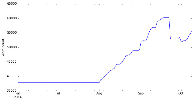
This shows the total word count of my thesis over time. I didn’t have the idea of writing this code until well into my PhD, so the time series starts in June 2014 when I was busy working on the practical side of my PhD. By that point I had already written some chapters (such as the literature review), but I didn’t really write anything else until early August (exactly the 1st August, as it happens). I then wrote quite steadily until my word count peaked on the 18th September, around the time that I submitted my final draft to my supervisors. The decrease after that was me removing a number of ‘less useful’ bits on advice from them!
Overall, I wrote 22,317 words between those two dates (a period of 48 days), which equates to an average of 464 words a day. However, on 22 of those days I wrote nothing – so on days that I actually wrote, I wrote an average of 858 words. My maximum number of words written in one day was 2,516, and the minimum was was -7,139 (when I removed a lot!). The minimum-non-zero was 5 words…that must have been a day when I was lacking in inspiration!
Some interesting graphs
One thing that I thought would be interesting would be to look at the total number of words I wrote each day of the week:
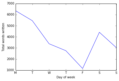
This shows a very noticeable tailing off as the week goes on, and then a peak again on Saturday. However, as this is a sum over the whole period it may hide a lot of interesting patterns. To see these, we can plot a heatmap showing the total number of words written each day of each week:
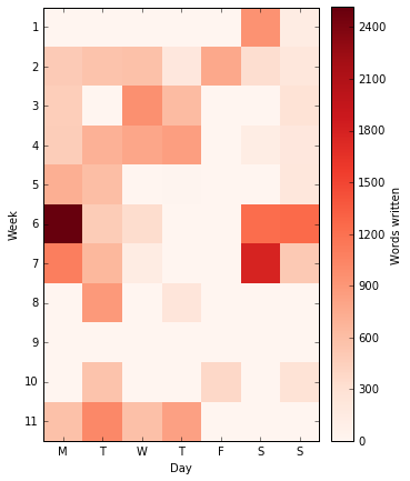
It seems like weeks 6 and 7 were very productive, and things tailed off gradually over the whole period, until the last week when they suddenly increased again (note that some of the very high values were when I copied things I’d written elsewhere into my main thesis documents).
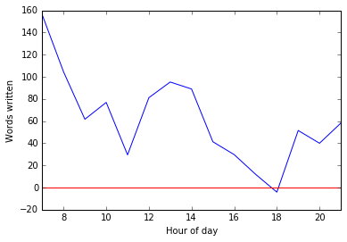
Looking at the number of words written over each hourly period is very easy in Pandas by grouping by the hour and then applying the ohlc function (Open-High-Low-Close), and then subtracting the Open value (number of words at the start of the hour) from the Close value (number of words at the end of the hour). Again, we can look at the total number of words written in each hour – summed across the whole period:
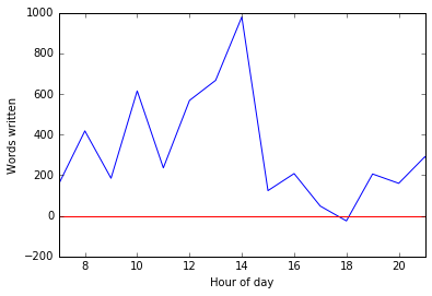
This shows that I had a big peak just after lunchtime (I tend to take a fairly early lunch around 12:00 or 12:30), with some peaks before breakfast (around 8:00) and after breakfast (10:00) – and similarly around the time of my evening meal (18:00), and then increasing as a bit of late work before bed. Of course, this shows the total contribution of each of these hours across the whole writing period, and doesn’t take into account how often I actually did any writing during these periods.
To see that we need to look at the mean number of words written during each hourly period:
This still shows a bit of a peak around lunchtime, but shows that by far my most productive time was early in the morning. Basically, when I wrote early in the morning I got a lot written, but I didn’t write early in the morning very often!
As before, we can look at this in more detail in a heatmap, in this instance by both hour of the day and day of the week:
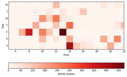
You can really start to see my schedule here. For example, I rarely wrote much on Sunday mornings because I was at church, but wrote quite effectively once I got back from work. I wrote very little around my evening meal time, and wrote very little on Monday mornings or Friday afternoons – which makes sense!
So, I hope you enjoyed this little tour through my thesis writing. All of the code for grabbing the versions from Dropbox is available on Github, along with a (very badly-written and badly-documented) notebook.
If you found this post useful, please consider buying me a coffee.
This post originally appeared on Robin's Blog.
Categorised as: Academic, LaTeX, Programming, Python, Remote Sensing
[…] retrieve the latest version of a file. I’ve used the Dropbox API from Python before (see my post about analysing my thesis-writing timeline with Dropbox) and it’s pretty easy. In fact, you […]