If someone wants to see how many times my work has been referenced, they’d probably go and look at my citation statistics, for example on my Google Scholar profile. At the time of writing, that shows that I have 16 citations overall, and a h-index of 2. However, I don’t think this tells the whole story.
Specifically, it only counts references to academic papers, books or conference proceedings (‘traditionally-citable items’), and it doesn’t take into account the far wider use of some of these items beyond traditional citations in other papers, books or conference proceedings. This misses out a lot of uses of my work – many of which are uses that I think are actually important (possibly more important than citations in other academic work).
(Please note that I’m not trying to point to other non-traditional references because I feel that my citation count is "too low", and I’m also not trying to say that a mention of my website URL is equivalent of a citation of my paper in another journal article – but I think these things should be taken into account, and it is hard to do so at the moment).
Anyway, I’ve been doing some investigation into some of the other uses of my work – mostly using various Google and Google Scholar searches – and I’ve found a lot of non-traditional references, some of which I didn’t know about before. For example:
RTWTools (my set of extensions for ENVI) has been used in three journal articles (including in Global and Planetary Change and Remote Sensing), a government report, and a MSc thesis
VanHOzone (my, very simple, implementation of the van Heuklon ozone model) has been used in a MSc thesis
Finally, my FreeGISData website has been referenced a lot, in at least six journal articles, four books or book chapters (including one non-academic book), a couple of subject magazines, two PhD theses and at least one MOOC course.
A full list of non-traditional references to my work is available here, but I hope you’ll agree that – although they are not traditional references in traditional academic works – these uses and applications of my work are important, and show a real impact – often beyond the academic community.
I’m supervising an MSc student for her thesis this summer, and the work she’s doing with me is going to involve a fair amount of programming, in the context of remote sensing & GIS processing. She’s got experience programming in IDL from a programming course during the taught part of her Masters, but has no experience of Python.
I’ve just sent her an email with links to some useful resources, but in the spirit of Matt Might’s Blog tips for busy academics, I thought it would be worth doing a ‘reply to public’, and putting the list of resources here. So, here goes…
Software Carpentry Python course:- this is designed for people new to programming, so some of it will be very easy for you. However, it takes you through a good example of scientific programming with Python, including plotting graphs and dealing with arrays. I suggest that you use the Jupyter Notebook to run through this – there are instructions on how to do that in the course, and there is a brief intro to the notebook in this YouTube video (start at approx 3 minutes – the stuff before that is irrelevant for you)
Lewis’s Scientific Programming for RS course (from UCL): – The most useful bits will probably be Python 101, Plotting and Numerical Python and Geospatial Data. Click the ‘Course Notes’ under each section to see the detailed notes.
Python Scripting with Spatial Data is also good – it gives a good intro to Python, and then covers spatial analysis using GDAL and RIOS (we won’t be using RIOS, but the GDAL stuff is good).
Geoprocessing with Python using Open Source GIS: This is a very good set of slides and tutorials – along with assignments, homework tasks and solutions – from a course run at Utah State University. Unfortunately it is now very old – it was written in 2008/9 – and so it refers to a number of out of date things (such as the ‘numeric’ library for Python, which has been replaced by numpy). A lot of the GDAL content is still useful though – for example, this set of slides on reading raster data with GDAL is pretty good.
There are various good tutorials from conferences such as SciPy (Scientific Python) and FOSS4G (Free and Open Source Software for Geospatial). For example, you can watch a video of a three-hour tutorial from SciPy 2015 called Geospatial Data with Open Source tools in Python, and you can find the slides and other resources here. This goes into quite a lot of depth, and new Python programmers may find it all quite daunting – but it demonstrates the nice modern ways of doing things (using libraries like Fiona and rasterio) rather than the less-nice and lower-level GDAL library.
Another couple of resources (suggested by Chris Holden in the comments – thanks!) are the WUR Geoscripting resources, which start with R and then moves on to Python, and his own Open Source Geoprocessing tutorial, which covers GDAL and OGR, and demonstrates how to calculate NDVI and even goes as far as land cover classification.
There are also a few useful resources for switching from IDL to Python. Specifically:
A Numpy reference for IDL users: (Numpy is the Python library that provides functions to manipulate arrays – unlike IDL, this isn’t included by default in Python – but it does come with the Anaconda distribution I mentioned above).
I wrote a blog post comparing a set of ‘Ten Little Programs’ in IDL with equivalents in Python, which should give you an idea of the similarities and differences, and how you can translate some of your code.
This is a very short list of a few resources – I’m sure there are some better ones out there, and so please let me know if you’ve got any recommendations!
As part of my fellowship with the Software Sustainability Institute, I’ve written an article on Software Sustainability in Remote Sensing. This article was originally written a couple of years ago and it never quite got around to being published. However, I have recently updated it, and it’s now been posted on the SSI’s blog. I’ve also ‘reblogged it’ below: it is a long read, but hopefully you’ll agree that it is worth it.
If anyone reading this is also interested in software sustainability in remote sensing, and identifies with some of the issues raised below then please get in touch! I’d love to discuss it with you and see what we can do to improve things.
1. What is remote sensing?
Remote sensing broadly refers to the acquisition of information about an object remotely (that is, with no physical contact). The academic field of remote sensing, however, is generally focused on acquiring information about the Earth (or other planetary bodies) using measurements of electromagnetic radiation taken from airborne or satellite sensors. These measurements are usually acquired in the form of large images, often containing measurements in a number of different parts of the electromagnetic spectrum (for example, in the blue, green, red and near-infrared), known as wavebands. These images can be processed to generate a huge range of useful information including land cover, elevation, crop health, air quality, CO2 levels, rock type and more, which can be mapped easily over large areas. These measurements are now widely used operationally for everything from climate change assessments (IPCC, 2007) to monitoring the destruction of villages in Darfur (Marx and Loboda, 2013) and the deforestation of the Amazon rainforest (Kerr and Ostrovsky, 2003).
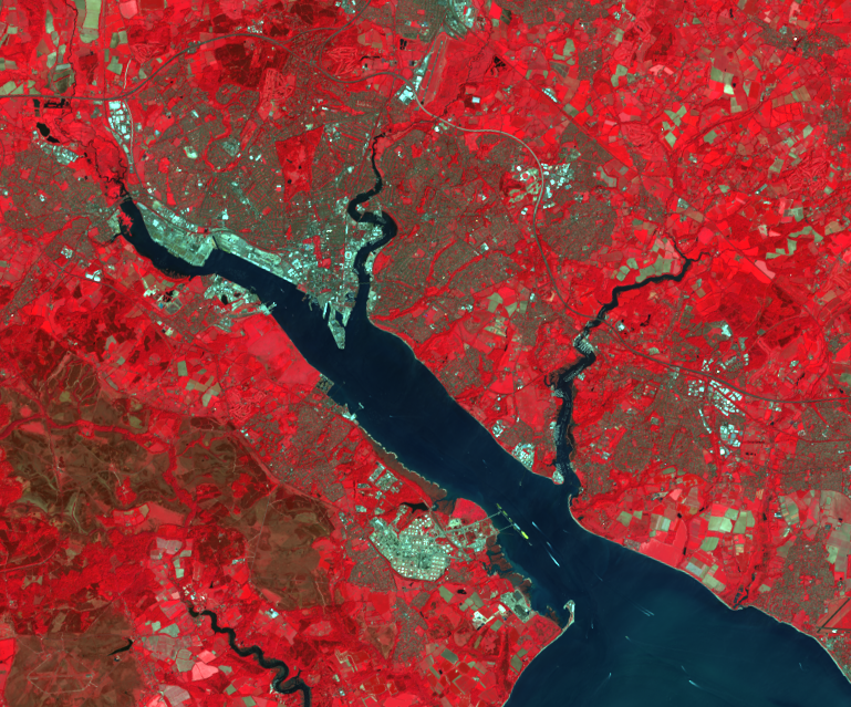
Figure 1: Landsat 8 image of Southampton, UK shown as a false-colour composite using the Near-Infrared, Red and Green bands. Vegetation is bright red, heathland and bare ground is beige/brown, urban areas are light blue, and water is dark blue.
The field, which crosses the traditional disciplines of physics, computing, environmental science and geography, developed out of air photo interpretation work during World War II, and expanded rapidly during the early parts of the space age. The launch of the first Landsat satellite in 1972 provided high-resolution images of the majority of the Earth for the first time, producing repeat images of the same location every 16 days at a resolution of 60m. In this case, the resolution refers to the level of detail, with a 60m resolution image containing measurements for each 60x60m area on the ground. Since then, many hundreds of further Earth Observation satellites have been launched which take measurements in wavelengths from ultra-violet to microwave at resolutions ranging from 50km to 40cm. One of the most recent launches is that of Landsat 8, which will contribute more data to an unbroken record of images from similar sensors acquired since 1972, now at a resolution of 30m and with far higher quality sensors. The entire Landsat image archive is now freely available to everyone – as are many other images from organisations such as NASA and ESA – a far cry from the days when a single Landsat image cost several thousands of dollars.
2. You have to use software
Given that remotely sensed data are nearly always provided as digital images, it is essential to use software to process them. This was often difficult with the limited storage and processing capabilities of computers in the 1960s and 1970s – indeed, the Corona series of spy satellites operated by the United States from 1959 to 1972 used photographic film which was then sent back to Earth in a specialised ‘re-entry vehicle’ and then developed and processed like standard holiday photos!
However, all civilian remote-sensing programs transmitted their data to ground stations on Earth in the form of digital images, which then required processing by both the satellite operators (to perform some rudimentary geometric and radiometric correction of the data) and the end-users (to perform whatever analysis they wanted from the images).
In the early days of remote sensing, computers didn’t even have the ability to display images onscreen, and the available software was very limited (see Figure 2a). Nowadays remote sensing researchers use a wide range of proprietary and open-source software, which can be split into four main categories:
Specialist remote-sensing image processing software, such as ENVI, Erdas IMAGINE, eCogniton, Opticks and Monteverdi
Geographical Information System software which provides some remote-sensing processing functionality, such as ArcGIS, IDRISI, QGIS and GRASS
Other specialist remote-sensing software, such as SAMS for processing spectral data, SPECCHIO for storing spectral data with metadata, DART (Gastellu-Etchegorry et al., 1996) for simulating satellite images and many numerical models including 6S (Vermote et al., 1997), PROSPECT and SAIL (Jacquemoud, 1993).
General scientific software, including numerical data processing tools, statistical packages and plotting packages.
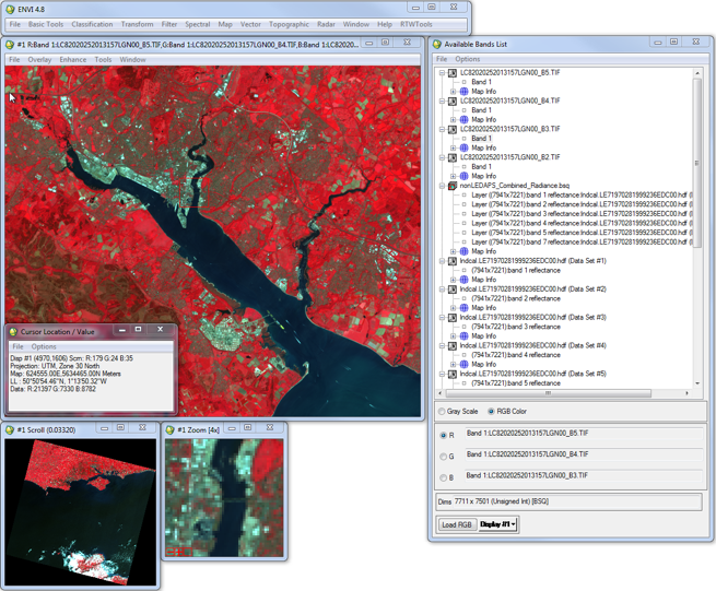
Figure 2: Remote sensing image processing in the early 1970s (a) and 2013 (b). The 1970s image shows a set of punched cards and an ‘ASCII-art’ printout of a Landsat image of Southern Italy, produced by E. J. Milton as part of his PhD. The 2013 image shows the ENVI software viewing a Landsat 8 image of Southampton on a Windows PC
I surveyed approximately forty people at the Remote Sensing and Photogrammetry Society’s Annual Student Meeting 2013 to find out how they used software in their research, and this produced a list of 19 pieces of specialist software which were regularly used by the attendees, with some individual respondents regularly using over ten specialist tools.
Decisions about which software to use are often based on experience gained through university-level courses. For example, the University of Southampton uses ENVI and ArcGIS as the main software in most of its undergraduate and MSc remote sensing and GIS courses, and many of its students will continue to use these tools significantly for the rest of their career. Due to the limited amount of teaching time, many courses only cover one or two pieces of specialist software, thus leaving students under-exposed to the range of tools which are available in the field. There is always a danger that students will learn that tool rather than the general concepts which will allow them to apply their knowledge to any software they might need to use in the future
I was involved in teaching a course called Practical Skills in Remote Sensing as part of the MSc in Applied Remote Sensing and GIS at the University of Southampton which tried to challenge this, by introducing students to a wide range of proprietary and open-source software used in remote sensing, particularly software which performs more specialist tasks than ENVI and ArcGIS. Student feedback showed that they found this very useful, and many went on to use a range of software in their dissertation projects.
2.1 Open Source Software
In the last decade there has been huge growth in open-source GIS software, with rapid developments in tools such as GIS (a GIS display and editing environment with a similar interface to ArcGIS) and GRASS (a geoprocessing system which provides many functions for processing geographic data and can also be accessed through GIS). Ramsey (2009) argues that the start of this growth was caused by the slowness of commercial vendors to react to the growth of online mapping and internet delivery of geospatial data, and this created a niche for open-source software to fill. Once it had a foothold in this niche, open-source GIS software was able to spread more broadly, particularly as many smaller (and therefore more flexible) companies started to embrace GIS technologies for the first time.
Unfortunately, the rapid developments in open-source GIS software have not been mirrored in remote sensing image processing software. A number of open-source GIS tools have specialist remote sensing functionality (for example, the i.* commands in GRASS), but as the entire tool is not focused on remotely sensed image processing they can be harder to use than tools such as ENVI. Open-source remote sensing image processing tools do exist (for example, Opticks, OrfeoToolbox, OSSIM, ILWIS and InterImage), but they tend to suffer from common issues for small open-source software projects, specifically: poor documentation; complex and unintuitive interfaces; and significant unfixed bugs.
In contrast, there are a number of good open-source non-image-based remote sensing tools, particularly those used for physical modelling (for example, 6S (Vermote et al., 1997), PROSPECT and SAIL (Jacquemoud, 1993)), processing of spectra (SAMS and SPECCHIO (Bojinski et al., 2003; Hueni et al., 2009)), and as libraries for programmers (GDAL, Proj4J).
Open source tools are gradually becoming more widely used within the field, but their comparative lack of use amongst some students and researchers compared to closed-source software may be attributed to their limited use in teaching. However, organisations such as the Open Source Geospatial Laboratories (OSGL:www.osgeo.org) are helping to change this, through collating teaching materials based on open-source GIS at various levels, and there has been an increase recently in the use of tools such as Quantum GIS for introductory GIS teaching.
3. Programming for remote sensing
There is a broad community of scientists who write their own specialist processing programs within the remote sensing discipline, with 80% of the PhD students surveyed having programmed as part of their research. In many disciplines researchers are arguing for increased use and teaching of software, but as there is no real choice as to whether to use software in remote sensing, it is the use and teaching of programming that has become the discussion ground.
The reason for the significantly higher prevalence of programming in remote sensing compared to many other disciplines is that much remote sensing research involves developing new methods. Some of these new methods could be implemented by simply combining functions available in existing software, but most non-trivial methods require more than this. Even if the research is using existing methods, the large volumes of data used in many studies make processing using a GUI-based tool unattractive. For example, many studies in remote sensing use time series of images to assess environmental change (for example, deforestation or increases in air pollution) and, with daily imagery now being provided by various sensors, these studies can regularly use many hundreds of images. Processing all of these images manually would be incredibly time-consuming, and thus code is usually written to automate this process. Some processing tools provide ‘macro’ functionality which allow common tasks to be automated, but this is not available in all tools (for example, ENVI) and is often very limited. I recently wrote code to automate the downloading, reprojecting, resampling and subsetting of over 7000 MODIS Aerosol Optical Thickness images, to create a dataset of daily air pollution levels in India over the last ten years: creating this dataset would have been impossible by hand!
The above description suggests two main uses of programming in remote sensing research:
Writing code for new methods, as part of the development and testing of these methods
Writing scripts to automate the processing of large volumes of data using existing methods
3.1 Programming languages: the curious case of IDL and the growth of Python
The RSPSoc questionnaire respondents used languages as diverse as Python, IDL, C, FORTRAN, R, Mathematica, Matlab, PHP and Visual Basic, but the most common of these were Matlab, IDL and Python. Matlab is a commercial programming language which is commonly used across many areas of science, but IDL is generally less well-known, and it is interesting to consider why this language has such a large following within remote sensing.
IDL’s popularity stems from the fact that the ENVI remote sensing software is implemented in IDL, and exposes a wide range of its functionality through an IDL Application Programming Interface (API). This led to significant usage of IDL for writing scripts to automate processing of remotely-sensed data, and the similarity of IDL to Fortran (particularly in terms of its array-focused nature) encouraged many in the field to embrace it for developing new methods too. Although first developed in 1977, IDL is still actively developed by its current owner (Exelis Visual Information Solutions) and is still used by many remote sensing researchers, and taught as part of MSc programmes at a number of UK universities, including the University of Southampton.
However, I feel that IDL’s time as one of the most-used languages in remote sensing is coming to an end. When compared to modern languages such as Python (see below), IDL is difficult to learn, time-consuming to write and, of course, very expensive to purchase (although an open-source version called GDL is available, it is not compatible with the ENVI API, and thus negates one of the main reasons for remote sensing scientists to use IDL).
Python is a modern interpreted programming language which has an easy-to-learn syntax – often referred to as ‘executable pseudocode’. There has been a huge rise in the popularity of Python in a wide range of scientific research domains over the last decade, made possible by the development of the numpy (‘numerical python’ (Walt et al., 2011)), scipy (‘scientific python’ (Jones et al., 2001)) and matplotlib (‘matlab-like plotting’ (Hunter, 2007)) libraries. These provide efficient access to and processing of arrays in Python, along with the ability to plot results using a syntax very similar to Matlab. In addition to these fundamental libraries, over two thousand other scientific libraries are available at the Python Package Index (http://pypi.python.org), a number of which are specifically focused on remote-sensing.
Remote sensing data processing in Python has been helped by the development of mature libraries of code for performing common tasks. These include the Geospatial Data Abstraction Library (GDAL) which provides functions to load and save almost any remote-sensing image format or vector-based GIS format from a wide variety of programming languages including, of course, Python. In fact, a number of the core GDAL utilities are now implemented using the GDAL Python interface, rather than directly in C++. Use of a library such as GDAL gives a huge benefit to those writing remote-sensing processing code, as it allows them to ignore the details of the individual file formats they are using (whether they are GeoTIFF files, ENVI files or the very complex Erdas IMAGINE format files) and treat all files in exactly the same way, using a very simple API which allows easy loading and saving of chunks of images to and from numpy arrays.
Another set of important Python libraries used by remote-sensing researchers are those originally focused on the GIS community, including libraries for manipulating and processing vector data (such as Shapely) and libraries for dealing with the complex mathematics of projections and co-ordinate systems and the conversion of map references between these (such as the Proj4 library, which has APIs for a huge range of languages). Just as ENVI exposes much of its functionality through an IDL API; ArcGIS, Quantum GIS, GRASS and many other tools expose their functionality through a Python API. Thus, Python can be used very effectively as a ‘glue language’ to join functionality from a wide range of tools together into one coherent processing hierarchy.
A number of remote-sensing researchers have also released very specialist libraries for specific sub-domains within remote-sensing. Examples of this include the Earth Observation Land Data Assimilation System (EOLDAS) developed by Paul Lewis (Lewis et al., 2012), and the Py6S (Wilson, 2012) andPyProSAIL (Wilson, 2013) libraries which I have developed, which provide a modern programmatic interface to two well-known models within the field: the 6S atmospheric radiative transfer model and the ProSAIL vegetation spectral reflectance model.
Releasing these libraries – along with other open-source remote sensing code – has benefited my career, as it has brought me into touch with a wide range of researchers who want to use my code, helped me to develop my technical writing skills and also led to the publication of a journal paper. More importantly than any of these though, developing the Py6S library has given me exactly the tool that I need to do my research. I don’t have to work around the features (and bugs!) of another tool – I can implement the functions I need, focused on the way I want to use them, and then use the tool to help me do science. Of course, Py6S and PyProSAIL themselves rely heavily on a number of other Python scientific libraries – some generic, some remote-sensing focused – which have been realised by other researchers.
The Py6S and PyProSAIL packages demonstrate another attractive use for Python: wrapping legacy code in a modern interface. This may not seem important to some researchers – but many people struggle to use and understand models written in old languages which cannot cope with many modern data input and output formats. Python has been used very successfully in a number of situations to wrap these legacy codes and provide a ‘new lease of life’ for tried-and-tested codes from the 1980s and 1990s.
3.2Teaching programming in remote sensing
I came into the field of remote sensing having already worked as a programmer, so it was natural for me to use programming to solve many of the problems within the field. However, many students do not have this prior experience, so rely on courses within their undergraduate or MSc programmes to introduce them both to the benefits of programming within the field, and the technical knowledge they need to actually do it. In my experience teaching on these courses, the motivation is just as difficult as the technical teaching – students need to be shown why it is worth their while to learn a complex and scary new skill. Furthermore, students need to be taught how to program in an effective, reproducible manner, rather than just the technical details of syntax.
I believe that my ability to program has significantly benefited me as a remote-sensing researcher, and I am convinced that more students should be taught this essential skill. It is my view that programming must be taught far more broadly at university: just as students in disciplines from Anthropology to Zoology get taught statistics and mathematics in their undergraduate and masters-level courses, they should be taught programming too. This is particularly important in a subject such as remote sensing where programming can provide researchers with a huge boost in their effectiveness and efficiency. Unfortunately, where teaching is done, it is often similar to department-led statistics and mathematics courses: that is, not very good. Outsourcing these courses to the Computer Science department is not a good solution either – remote sensing students do not need a CS1-style computer science course, they need a course specifically focused on programming within remote sensing.
In terms of remote sensing teaching, I think it is essential that a programming course (preferably taught using a modern language like Python) is compulsory at MSc level, and available at an undergraduate level. Programming training and support should also be available to researchers at PhD, Post-Doc and Staff levels, ideally through some sort of drop-in ‘geocomputational expert’ service.
4. Reproducible research in remote sensing
Researchers working in ‘wet labs’ are taught to keep track of exactly what they have done at each step of their research, usually in the form of a lab notebook, thus allowing the research to be reproduced by others in the future. Unfortunately, this seems to be significantly less common when dealing with computational research – which includes most research in remote sensing. This has raised significant questions about the reproducibility of research carried out using ‘computational laboratories’, which leads to serious questions about the robustness of the science carried out by researchers in the field – as reproducibility is a key distinguishing factor of scientific research from quackery (Chalmers, 1999).
Reproducibility is where the automating of processing through programming really shows its importance: it is very hard to document exactly what you did using a GUI tool, but an automated script for doing the same processing can be self-documenting. Similarly, a page of equations describing a new method can leave a lot of important questions unanswered (what happens at the boundaries of the image? how exactly are the statistics calculated?) which will be answered by the code which implements the method.
A number of papers in remote sensing have shown issues with reproducibility. For example, Saleska et al. (2007) published a Science paper stating that the Amazon forest increased in photosynthetic activity during a widespread drought in 2005, and thus suggested that concerns about the response of the Amazon to climate change were overstated. However, after struggling to reproduce this result for a number of years, Samanta et al. (2010) eventually published a paper showing that the exact opposite was true, and that the spurious results were caused by incorrect cloud and aerosol screening in the satellite data used in the original study. If the original paper had provided fully reproducible details on their processing chain – or even better, code to run the entire process – then this error would likely have been caught much earlier, hopefully during the review process.
I have personally encountered problems reproducing other research published in the remote sensing literature – including the SYNTAM method for retrieving Aerosol Optical Depth from MODIS images (Tang et al., 2005), due to the limited details given in the paper, and the lack of available code, which has led to significant wasted time. I should point out, however, that some papers in the field deal with reproducibility very well. Irish et al. (2000) provide all of the details required to fully implement their revised version of the Landsat Automatic Cloud-cover Assessment Algorithm (ACCA), mainly through a series of detailed flowcharts in their paper. The release of their code would have saved me re-implementing it, but at least all of the details were given.
5. Issues and possible solutions
The description of the use of software in remote sensing above has raised a number of issues, which are summarised here:
There is a lack of open-source remote-sensing software comparable to packages such as ENVI or Erdas Imagine. Although there are some tools which fulfil part of this need, they need an acceleration in development in a similar manner to Quantum GIS to bring them to a level where researchers will truly engage. There is also a serious need for an open-source tool for Object-based Image Analysis, as the most-used commercial tool for this (eCognition) is so expensive that it is completely unaffordable for many institutions.
There is a lack of high-quality education in programming skills for remote-sensing students at undergraduate, masters and PhD levels.
Many remote sensing problems are conceptually easy to parallelise (if the operation on each pixel is independent then the entire process can be parallelised very easily), but there are few tools available to allow serial code to be easily parallelised by researchers who are not experienced in high performance computing.
Much of the research in the remote sensing literature is not reproducible. This is a particular problem when the research is developing new methods or algorithms which others will need to build upon. The development of reproducible research practices in other disciplines has not been mirrored in remote sensing, as yet.
Problems 2 & 4 can be solved by improving the education and training of researchers – particularly students – and problems 1 & 3 can be solved by the development of new open-source tools, preferably with the involvement of active remote sensing researchers. All of these solutions, however, rely on programming being taken seriously as a scientific activity within the field, as stated by the Science Code Manifesto (http://sciencecodemanifesto.org).
6. Advice
The first piece of advice I would give any budding remote sensing researcher is learn to program! It isn’t that hard – honestly! – and the ability to express your methods and processes in code will significantly boost your productivity, and therefore your career.
Once you’ve learnt to program, I would have a few more pieces of advice for you:
Script and code things as much as possible, rather than using GUI tools. Graphical User Interfaces are wonderful for exploring data – but by the time you click all of the buttons to do some manual processing for the 20th time (after you’ve got it wrong, lost the data, or just need to run it on another image) you’ll wish you’d coded it.
Don’t re-invent the wheel. If you want to do an unsupervised classification then use a standard algorithm (such as ISODATA or K-means) implemented through a robust and well-tested library (like the ENVI API, or scikit-learn) – there is no point wasting your time implementing an algorithm that other people have already written for you!
Try and get into the habit of documenting your code well – even if you think you’ll be the only person who looks at it, you’ll be surprised what you can forget in six months!
Don’t be afraid to release your code – people won’t laugh at your coding style, they’ll just be thankful that you released anything at all! Try and get into the habit of making research that you publish fully reproducible, and then sharing the code (and the data if you can) that you used to produce the outputs in the paper.
References
Bojinski, S., Schaepman, M., Schläpfer, D., Itten, K., 2003. SPECCHIO: a spectrum database for remote sensing applications. Comput. Geosci. 29, 27-38.
Chalmers, A.F., 1999. What is this thing called science? Univ. of Queensland Press.
Hueni, A., Nieke, J., Schopfer, J., Kneubühler, M., Itten, K.I., 2009. The spectral database SPECCHIO for improved long-term usability and data sharing. Comput. Geosci. 35, 557-565.
Irish, R.R., 2000. Landsat 7 automatic cloud cover assessment, in: AeroSense 2000. International Society for Optics and Photonics, pp. 348-355.
Jacquemoud, S., 1993. Inversion of the PROSPECT+ SAIL canopy reflectance model from AVIRIS equivalent spectra: theoretical study. Remote Sens. Environ. 44, 281292.
Jones, E., Oliphant, T., Peterson, P., others, 2001. SciPy: Open source scientific tools for Python.
Kerr, J.T., Ostrovsky, M., 2003. From space to species: ecological applications for remote sensing. Trends Ecol. Evol. 18, 299-305. doi:10.1016/S0169-5347(03)00071-5
Lewis, P., Gómez-Dans, J., Kaminski, T., Settle, J., Quaife, T., Gobron, N., Styles, J., Berger, M., 2012. An Earth Observation Land Data Assimilation System (EO-LDAS). Remote Sens. Environ. 120, 219-235. doi:10.1016/j.rse.2011.12.027
Marx, A.J., Loboda, T.V., 2013. Landsat-based early warning system to detect the destruction of villages in Darfur, Sudan. Remote Sens. Environ. 136, 126-134. doi:10.1016/j.rse.2013.05.006
Ramsey, P., 2009. Geospatial: An Open Source Microcosm. Open Source Bus. Resour.
Saleska, S.R., Didan, K., Huete, A.R., Da Rocha, H.R., 2007. Amazon forests green-up during 2005 drought. Science 318, 612-612.
Samanta, A., Ganguly, S., Hashimoto, H., Devadiga, S., Vermote, E., Knyazikhin, Y., Nemani, R.R., Myneni, R.B., 2010. Amazon forests did not green-up during the 2005 drought. Geophys. Res. Lett. 37, L05401.
Tang, J., Xue, Y., Yu, T., Guan, Y., 2005. Aerosol optical thickness determination by exploiting the synergy of TERRA and AQUA MODIS. Remote Sens. Environ. 94, 327-334. doi:10.1016/j.rse.2004.09.013
Vermote, E.F., Tanre, D., Davis, J.L., Herman, M., Morcette, J.J., 1997. Second Simulation of the Satellite Signal in the Solar Spectrum, 6S: an overview. IEEE Trans. Geosci. Remote Sens. 35, 675-686. doi:10.1109/36.581987
Walt, S. van der, Colbert, S.C., Varoquaux, G., 2011. The NumPy Array: A Structure for Efficient Numerical Computation. Comput. Sci. Eng. 13, 22-30. doi:10.1109/MCSE.2011.37
Wilson, R.T., 2013. PyProSAIL.
Wilson, R.T., 2012. Py6S: A Python interface to the 6S Radiative Transfer Model. Comput. Geosci. 51, 166-171.
So, first things first: many of the regular readers of my blog may not know this, but I have recently started using a wheelchair:
(This was my first time out in my new electric wheelchair, hence the look of concentration on my face!)
If you’re a regular reader of my blog and have just thought "Wow – surely he can’t be in a wheelchair, because he’s a good programmer, and a (moderately successful) academic!" then please read to the end of this blog, and ideally some of the rest of the BADD posts!
I’m not going to go into all of the medical stuff here, but basically I can walk a bit (upto about 100-150m), but anything more than that will utterly exhaust me. This situation is not ideal, it has only happened in the last six months to a year or so, and it has taken me a while to adjust emotionally to "being disabled", but – and this is the important thing – a wheelchair is, for me, a huge enabler. It gives me freedom, rather than restricting me.
My wheelchair doesn’t restrict me doing many things by its very nature (and in fact I can do many things that non-wheelchair-users can’t do, like carry very heavy loads, hold a baby on my lap while walking, and travel 10 miles at 4mph consistently) – but the design of the environments that I need to use on a day-to-day basis do restrict what I can do, as do the structure of the systems that I have to work within, and the opinions of some people.
I’m going to talk about things that are particularly related to my field of work: academia. I really don’t know how to organise this post, so I think I will just post a bulleted list of experiences, thoughts, observations etc. I’m trying not to ‘moan’ too much, but some of these experiences have really shocked me.
One other thing to bear in mind here is that many of these things are just because people "don’t think", not necessarily because they are deliberately being "anti-disabled people" – but in the end, the practical issues that result affect me the same amount regardless of the reason behind them.
So, on with my random list:
I was informed by the university insurance office that when travelling to a conference the university insurance would cover my electric wheelchair, but I would be required to cover the excess of £1500 if there was a claim. This was because it was a “personal item” and therefore treated the same as any other expensive personal item, such as a diamond ring. I’ve now managed to sort this – and there should be a new university-wide policy coming out soon – but sorting it required pestering HR, the Equality & Diversity team, the Insurance Office and my Faculty. Surely someone had travelled with a wheelchair before?!
I went to an Equality & Diversity event at the university with various panel discussions that didn’t touch on disability as an Equality/Diversity issue at all – the focus was entirely on gender, race and sexuality. I’m aware that there are probably more women in the university than disabled people (!), but actually if you take into account the statistics of the number of people who are disabled in some way then it must affect a large proportion of staff!
I went to a conference in Edinburgh which was held in a venue that was described as “fully-accessible”. The conference organisers (who, I want to state, did everything as they should have: checking with the venue about accessibility before booking the conference) were told that everything would be fine for me to attend in a wheelchair, and I was told the same thing when I phoned in advance to check. Just two examples from my three day conference should give you an idea of what it was like for me:
It took me about ten minutes to get, in my wheelchair, from the main conference room to the disabled toilet, and this involved going through four sets of doors. One of these doors was locked (and required a code to open), and I was originally told that I’d need to find a security guard to ask to open this door every time I wanted to go to the toilet! Umm…as an adult I’d rather not have to ‘ask permission’ to go to the toilet…so luckily my wife memorised the code! There were multiple times when other doors along the route were locked too. I felt like a second-class citizen just for wanting to go to the toilet!
After the conference dinner one evening I was told that there was “no step-free way for me to leave the venue”. I was somewhat confused by this, as I had entered the venue without using any steps…but it turned out that the main entrance gates were locked and “they couldn’t find the key”. After disappearing for ten minutes to try and find a key, their suggested solution was to carry me down some stairs and out of another exit.
The lifts in many university buildings are barely large enough to fit my (relatively small) wheelchair, meaning I have often got stuck half-in a lift…not a fun experience! There are other wonderful things about many university buildings and environments, including entrance ramps to buildings that are located at the bottom of a flight of stairs (why?!), disabled toilets that are only accessible through very heavy doors (almost impossible to push in a wheelchair), and the fact that the majority of the lecture theatres are not accessible for me as a lecturer!
It is often assumed that, as someone in a wheelchair, you must be a) a student, and b) need help. I’ve been stopped by people many times on campus and asked if I need directions, or help getting somewhere – despite the fact that I’ve been working on that campus for nearly 10 years now, and I don’t look much like a student. I don’t mind people offering to help (far from it) – but it shows an in-built assumption that I can’t be a staff member, I can’t know what I’m doing, and I must be a ‘helpless person’.
That’s just a few things I can think of off the top of my head. A few more generic points that I’d like to make are:
Why is it that at least 50% of the time, people who say that they will make some sort of "special arrangements" for you because of your disability do not actually do so?! I just can’t understand it! Examples include:
The hotel that booked an “adapted room” for me, except that I didn’t actually get given an adapted room because “they were all in use” (surely they knew that when booking me?!). They did manage to provide a stool for the shower, and the room was large enough to get my wheelchair into – but why on earth did this happen?
The special assistance person at Heathrow who just disappeared after giving me back my wheelchair, leaving me to try and wheel around all of the queues at passport control rather than going down the ‘medical lane’ (which I didn’t know existed)
and why is it that the organisations that are meant to support you are so often unable or unwilling to do that?! For example:
After spending four months going through the Access to Work scheme to try and get an electric wheelchair which I need for work (and which I was assessed as needing for work), I was rejected and told that I didn’t need it and wouldn’t be funded it. It’s called Access to Work and I needed my wheelchair to access work – it’s not that difficult (luckily my family offered to fund my wheelchair). I know the answer to this (it’s about government cuts), but I’m not going to go into a rant about the government here!
The university has a lot of support for disabled students (with a whole disability service, Disabled Students Allowance, the Counselling Service and so on), but nothing like that to help staff.
Everything just takes a huge amount longer, and none of the systems are designed to work well for people with disabilities. This ranges from travelling around the building (the lift in my building is hidden in the far corner and it takes a long time to wiggle around the corridors to get there), to booking events (most people just book a flight online: I have to have a half an hour phone call with the airline giving them pages of information on my wheelchair battery) to doing risk assessments (don’t get me started…). For someone who is working part-time anyway, this takes up a huge proportion of my time!
The combination of these examples – and many more that I can’t think of right now – is that I often feel like a second-class citizen, in academia, on campus, when travelling and so on. This isn’t right – but the silly thing is that it doesn’t take that much effort to change. Many of the examples given above could have been changed without much effort or much expenditure. Most of them are really simple: just don’t say anti-disability things, if you promise to do something then do it, add some chairs, prop the door open (or officially give me the code), don’t lie about the accessibility of your building, and so on. It’s not that hard!
Anyway, I’d like to end on a positive note, with an example of a conference that is doing pretty-much everything it can to be accessible and inclusive. It’s not actually an academic conference, it’s PyConUK 2016 – a conference on the Python programming language. When I read their diversity, accessibility and inclusion page I actually cried. The headline on that page says "You are a first-class citizen of our community", and then goes on to discuss what they have done in detail. I’ll let you read the page for the details, but basically they offer financial assistance, a free creche, a quiet room to relax away from the conference, step-free access, BSL interpreters, speech-to-text translation, and more. I’ve spoken to the organisers and thanked them for this, and after the conference I’m intending to ask them how much extra this inclusion work has added to their budget…and I suspect the answer will be "very little", but it will make such a huge difference to me and to many others.
This is a very brief post to explain how I managed to speed up the viewing (that is, listing of files/directories) in Samba shares accessed via OS X.
So, a bit of background: I have a file server at home which has some shared folders on it, shared using the SMB protocol. This is the ‘Windows File Sharing’ protocol, and is implemented using the Samba project on Linux.
OS X can access these folders, by opening Finder and selecting Go -> Connect to server (or pressing Cmd-K) and typing smb://SERVER and selecting the shared folder. However, you may find – as I did – that once you have connected to the shared folder, it takes a huge amount of time to list folders that contain a large number of files or subfolders (in my case, this was my photos backup folders). At times it took over five minutes to list the contents of a folder…far too long!
Anyway, with a bit of Googling and trial and error, I found that telling OS X to use version 1 of the SMB protocol seemed to speed this up significantly – and didn’t seem to have a significant impact on data transfer rates.
To force OS X to use v1 of the protocol, just create a file called ~/Library/Preferences/nsmb.conf, with the contents:
[default]

smb_neg=smb1_only
If you want to create this easily from the command line, you can just run the following command:
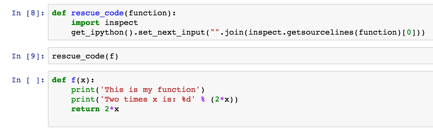
Jupyter (formerly known as IPython) notebooks are great – but have you ever accidentally deleted a cell that contained a really important function that you want to keep? Well, this post might help you get it back.
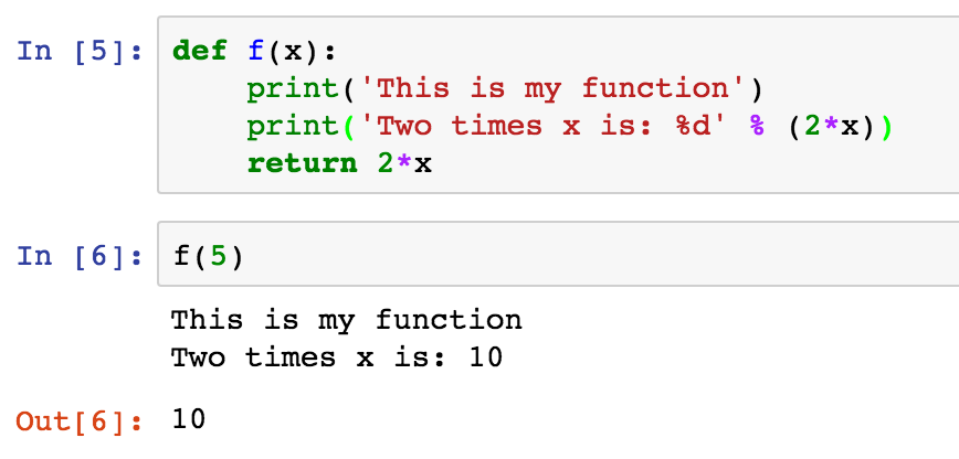
So, imagine you have a notebook with the following code:
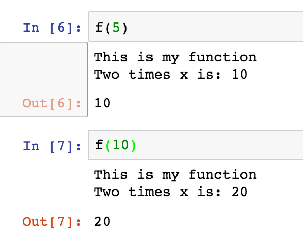
and then you accidentally delete the top cell, with the definition of your function…oops! Furthermore, you can’t find it in any of your ‘Checkpoints’ (look under the File menu). Luckily, your function is still defined…so you can still run it:
This is essential for what follows…because as the function is still defined, the Python interpreter still knows internally what the code is, and it gives us a way to get this out!
So, if you’re stuck and just want the way to fix it, then here it is:
Just call this as rescue_code(f), or whatever your function is, and a new cell should be created with the code of you function: problem solved! If you want to learn how it works then read on…
The code is actually very simple, inspect.getsourcelines(function) returns a tuple containing a list of lines of code for the function and the line of the source file that the code starts on (as we’re operating in a notebook this is always 1). We extract the 0th element of this tuple, then join the lines of code into one big string (the lines already have \n at the end of them, so we don’t have to deal with that. The only other bit is a bit of IPython magic to create a new cell below the current cell and set its contents….and that’s it!
I hope this is helpful to someone – I’m definitely going to keep this function in my toolkit.
Another instalment in my Previously Unpublicised Code series…this time RPiNDVI, my code for displaying live NDVI images from the Raspberry Pi NoIR camera.
It isn’t perfect, and it isn’t finished – but it does the job as a proof-of-concept. If you point the camera out of your window you should see high NDVI values (white) over vegetation, and low NDVI values (black) over various other things (particularly the sky!).
This is the point at which I would like to include a screenshot of the program running…but unfortunately I can’t actually find my Raspberry Pi to run it! (I guess that’s the problem with small computers…).
I can’t say the code is exceptionally exciting – it’s only about 100 lines – but it might be useful to someone. It demonstrates how to do real-time (or near-real-time) processing of video from the Raspberry Pi camera using OpenCV, and also has a few handy functions for doing contrast stretching of imagery and combining multiple images on a single display.
As always, the code is available at Github, along with a list of requirements – so have fun!
I wrote my PhD thesis in LaTeX, and stored all of the files in my Dropbox folder. Dropbox stores previous versions of your files – for up to 30 days if you are on their free plan. Towards the end of my PhD, I realised that I could write a fairly simple Python script that would grab all of these previous versions, which I could then use to do some interesting analyses. So – over a year after my thesis was submitted, I’ve finally got around to looking at the data.
I should point out here that this data comes from a sample size of one – and so if you’re writing a PhD thesis then don’t compare your speed/volume/length/whatever to me! So, with that disclaimer, on to how I did it, and what I found…
Getting the data
I wrote a nice simple class in Python to grab all previous versions of a file from Dropbox. It’s available in the DropboxBasedWordCount repo on Github – and can be used entirely independently from the LaTeX analysis that I did. It is really easy to use, just grab the DropboxDownloader.py file, install the Dropbox library (pip install Dropbox) and run something like this:
from DropboxDownloader import DropboxDownloader

# Initialise the object and give it the folder to store its downloads in
d = DropboxDownloader('/Users/robin/ThesisFilesDropboxLog')

# Download all available previous versions
d.download_history_for_files("/Users/robin/Dropbox/_PhD/_FinalThesis",  # Folder containing files to download
                             "*.tex",  # 'glob' string specifying files to download
                             "/Users/robin/Dropbox/")  # Path to your Dropbox folder
The code inside the DropboxDownloader class is actually quite simple – it basically just calls the revisions method of the DropboxClient object, does a bit of processing of filenames and timestamps, and then grabs the file contents with the get_file method, making sure to set the rev parameter appropriately.
Counting the words
Now we have a folder (or set of folders) full of files, we need to actually count the words in them. This will vary significantly depending on what typsetting system you’re using, but for LaTeX we can use the wonderful texcount. You’ll probably find it is installed automatically with your TeX distribution, and it has a very comprehensive set of documentation that I’ll let you go away and read…
For our purposes, we wanted a simple output of the total number of words in the file, so I ran it as:
texcount -brief -total -1 -sum file.tex
I ran this from Python using subprocess.Popen (farbetter than os.system!) for each file, combining the results into a Pandas DataFrame.
Doing the analysis
Now we get to the interesting bit: what can we find out about how I wrote my thesis. I’m not going to go into details about exactly how I did all of this, but I will occasionally link to useful Pandas or NumPy functions that I used.
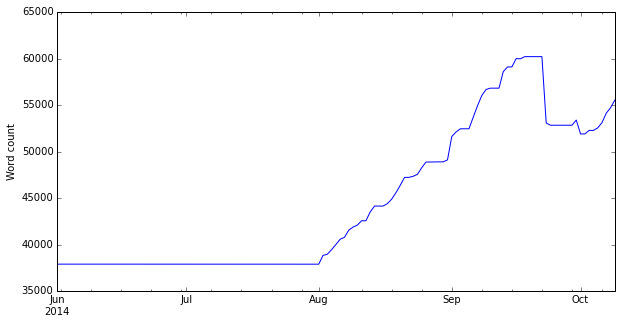
When you get hold of some data – particularly if it is time-series – then it is always good to plot it and see what it looks like. The pandas plot function makes this very easy – and we can easily get a plot like this:
This shows the total word count of my thesis over time. I didn’t have the idea of writing this code until well into my PhD, so the time series starts in June 2014 when I was busy working on the practical side of my PhD. By that point I had already written some chapters (such as the literature review), but I didn’t really write anything else until early August (exactly the 1st August, as it happens). I then wrote quite steadily until my word count peaked on the 18th September, around the time that I submitted my final draft to my supervisors. The decrease after that was me removing a number of ‘less useful’ bits on advice from them!
Overall, I wrote 22,317 words between those two dates (a period of 48 days), which equates to an average of 464 words a day. However, on 22 of those days I wrote nothing – so on days that I actually wrote, I wrote an average of 858 words. My maximum number of words written in one day was 2,516, and the minimum was was -7,139 (when I removed a lot!). The minimum-non-zero was 5 words…that must have been a day when I was lacking in inspiration!
Some interesting graphs
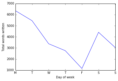
One thing that I thought would be interesting would be to look at the total number of words I wrote each day of the week:
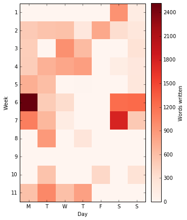
This shows a very noticeable tailing off as the week goes on, and then a peak again on Saturday. However, as this is a sum over the whole period it may hide a lot of interesting patterns. To see these, we can plot a heatmap showing the total number of words written each day of each week:
It seems like weeks 6 and 7 were very productive, and things tailed off gradually over the whole period, until the last week when they suddenly increased again (note that some of the very high values were when I copied things I’d written elsewhere into my main thesis documents).
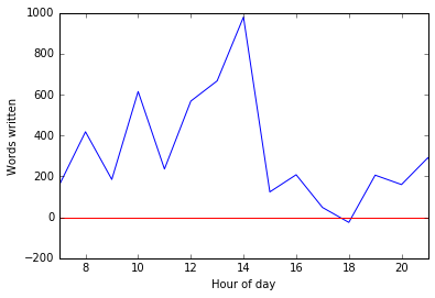
Looking at the number of words written over each hourly period is very easy in Pandas by grouping by the hour and then applying the ohlc function (Open-High-Low-Close), and then subtracting the Open value (number of words at the start of the hour) from the Close value (number of words at the end of the hour). Again, we can look at the total number of words written in each hour – summed across the whole period:
This shows that I had a big peak just after lunchtime (I tend to take a fairly early lunch around 12:00 or 12:30), with some peaks before breakfast (around 8:00) and after breakfast (10:00) – and similarly around the time of my evening meal (18:00), and then increasing as a bit of late work before bed. Of course, this shows the total contribution of each of these hours across the whole writing period, and doesn’t take into account how often I actually did any writing during these periods.
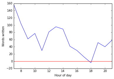
To see that we need to look at the mean number of words written during each hourly period:
This still shows a bit of a peak around lunchtime, but shows that by far my most productive time was early in the morning. Basically, when I wrote early in the morning I got a lot written, but I didn’t write early in the morning very often!
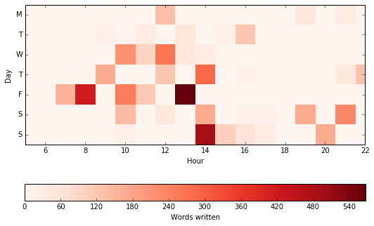
As before, we can look at this in more detail in a heatmap, in this instance by both hour of the day and day of the week:
You can really start to see my schedule here. For example, I rarely wrote much on Sunday mornings because I was at church, but wrote quite effectively once I got back from work. I wrote very little around my evening meal time, and wrote very little on Monday mornings or Friday afternoons – which makes sense!
So, I hope you enjoyed this little tour through my thesis writing. All of the code for grabbing the versions from Dropbox is available on Github, along with a (very badly-written and badly-documented) notebook.
Summary: When you type script.py at the Command Prompt on Windows, the Python executable used to run the script is not the first python.exe file found on your PATH, it is the the executable that is configured to run .py files when you double-click on them, which is configured in the registry.
I ran into a strange problem on Windows recently, when I was trying to run one of the GDAL command-line Python scripts (I think it was gdal_merge.py). I had installed GDAL in my conda environment, and gdal_merge.py was available on my PATH, but when I ran it I got an error saying that it couldn’t import the gdal module. This confused me a bit, so I did some more investigation.
I eventually ended up editing the gdal_merge.py script and adding a few lines at the top
This showed me that the script was being run by a completely different Python interpreter, with a completely separate site-packages folder – so it was hardly surprising that it couldn’t find the gdal library. It turns out that this ‘other’ Python interpreter was the one installed automatically by ArcGIS (hint: during the ArcGIS setup wizard, tell it to install Python to c:\ArcPython27, then it’s easy to tell which is which). But, how could this be, as I’d removed anything to do with the ArcGIS Python from my PATH…?
After a bit of playing around and Googling things, I found that when you type something like gdal_merge.py at the Command Prompt it doesn’t look on your PATH to find a python.exe file to execute the file with…instead it does the same thing as it would do if you double-clicked on the Python file in Explorer. This is kind of obvious in retrospect, but I spent a long time working it out!
The upshot of this is that if you want to change the Python installation that is used, then you need to change the Filetype Assocation for .py files. This can be done by editing the registry (look at HKEY_CLASSES_ROOT\Python.File\shell\open\command) or on the command-line using the ftype command (see here and here).
So, I really like the Jupyter notebook (formerly known as the IPython notebook), but I often find myself missing the ‘fancy’ features that ‘proper’ editors have. I particularly miss the amazing multiple cursor functionality of editors like Sublime Text and Atom.
I’ve known for a while that you can edit a cell in your default $EDITOR by running %%edit at the top of the cell – but I’ve recently found out that you can configure Jupyter to use Sublime Text-style keyboard shortcuts when editing cells in the notebook – all thanks to CodeMirror, the javascript-based text editor component that the Jupyter notebook uses. Brilliantly, this also brings with it the multiple-cursor functionality! So, you can get something like this:
So, how do you do this? It’s really simple.
Find your Jupyter configuration folder by running jupyter --config-dir
Open the custom.js file in the custom sub-folder in your favourite editor
Add the following lines to the bottom of the file
require(["codemirror/keymap/sublime", "notebook/js/cell", "base/js/namespace"],
    function(sublime_keymap, cell, IPython) {
        // setTimeout(function(){ // uncomment line to fake race-condition
        cell.Cell.options_default.cm_config.keyMap = 'sublime';
        var cells = IPython.notebook.get_cells();
        for(var cl=0; cl< cells.length ; cl++){
            cells[cl].code_mirror.setOption('keyMap', 'sublime');
        }

        // }, 1000)// uncomment  line to fake race condition
    }
);
That should be it – if you start a notebook now all of the Sublime Text shortcuts should be working!