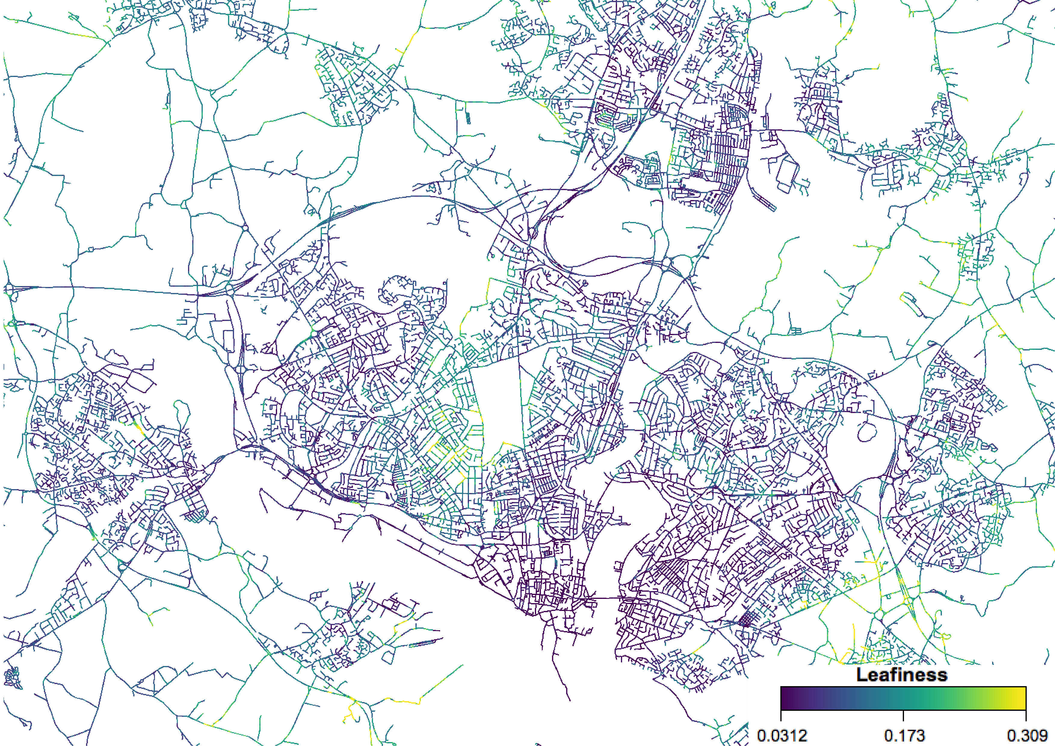
In the last post in this series, I showed some pretty maps of roadside leafiness, created by extracting NDVI values near roads – like this:
This time, I want to move away from pretty images to some numerical analysis – and also move from a local scale to a national scale.
My first question was: which is the leafiest place in the country?
Now, that question requires a bit of refining – firstly to work out what we mean by a "place". If we look in the countryside then we’re going to find very leafy roads – so we need to restrict this to urban areas. Luckily, the Office for National Statistics have produced a dataset that helps us here: the Built-Up Areas Boundary dataset. This data, from 2011, is automatically created from Ordnance Survey data, and consists of vector outlines of built-up areas in England. We can take these polygons and extract the average leafiness in each polygon and produce a map like this:
You can see here that lots of built-up areas are present, including many very small areas. You can also see that some areas are very large – built-up areas within a certain distance of each other are merged, which creates a ‘South Hampshire Built-Up Area’ which includes Southampton, Eastleigh, Chandlers Ford, Fareham, Gosport, Portsmouth and more. It’s rather frustrating from the perspective of our analysis, but I suppose it shows how built-up this area of South Hampshire is.
We can go ahead and export this aggregated leafiness data to CSV (I chose to aggregate using mean and median to compare them) to continue the analysis in Python. If you want to see how I analysed the CSV data then have a look at this notebook – but it’s fairly simple pandas analysis, and the main results are reproduced here.
So – which are the leafiest places in the country?
Name
Leafiness
Winchester
0.23
Northwich
0.18
Maidenhead
0.18
Heswall
0.17
Worcester
0.16
You can see that Winchester comes out top by a fair way. Winchester is probably the only one of these that I would have immediately thought of as very leafy – but that probably says more about my preconceptions than anything else. These were calculated using mean leafiness, but the top four stay the same, and the fifth entry is Great Malvern. I think that is likely an anomaly as the built-up area outline for Great Malvern actually includes Malvern Link, West Malvern, Colwall and a number of other smaller settlements nearby – and includes the green areas between these individual settlements.
The lowest areas are:
Name
Leafiness
Grays
0.05
Thanet
0.05
Greater London
0.06
Stevenage
0.06
Exeter
0.07
Embarassingly, I’d never heard of Grays – but it turns out it is on the banks of the Thames in East London, just east of the Dartford Crossing.
The most variable areas are:
Name
CV
Thanet
0.90
Felixstowe
0.67
Reading
0.64
Blackpool
0.62
Greater Manchester
0.60
and the least variable areas are:
Name
CV
Bath
0.22
Yeovil
0.23
Stafford
0.25
York
0.25
Durham
0.27
We can also plot mean against coefficient of variation, which allows us to examine where areas are placed when considering both the leafiness and the variability of this leafiness. The image below shows a static version of this graph – I actually produced an interactive version using my code to easily produce Bokeh plots with tooltips, and that interactive version can be found at the bottom of the notebook used to do the analysis.
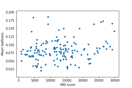
I also did a bit more analysis, extracting leafiness over all Lower Layer Super Output Areas (LSOAs) in Southampton, and joining the data with the Index of Multiple Deprivation from the 2011 census – aiming to discover if there is a link between leafiness and the deprivation of an area. Short answer: there isn’t – as the graph below demonstrates:
So, that’s the end of a fun bit of analysis – thanks to James O’Connor again for the idea.
If you just want to see some pretty maps of roadside leafiness then scroll down…otherwise, start at the top to find out how I did this.
I’ve recently started doing a little bit of satellite imaging work again, and started off with a project that was inspired by a post on James O’Connor’s blog. He posted about looking at the leafiness of streets in cities by extracting the NDVI (Normalized Difference Vegetation Index) within 20m of a road. He did this for Cleveland, Ohio using data from the Landsat 5 sensor, and produced a nice output map showing some interesting patterns.
This caught my interest, and I decided to see if I could scale up the analysis to larger areas. My go-to tool for doing simple but large-scale remote sensing work is Google Earth Engine – a free tool provided by Google which can easily process large volumes of satellite imagery stored on Google’s servers. To use this tool you have to be a ‘registered tester’, as the tool is not fully released yet, but it is easy to register to become a tester.
For this particular task I needed two datasets: some relatively high-resolution satellite imagery to use to calculate the NDVI, and some vector data of the road network. Conveniently, Google Earth Engine already contains datasets that fulfil these criteria: all of the Sentinel-2 data is in there, which provides visible and near-infrared bands at 10-30m resolution (depending on the band – the ones that we need for NDVI calculation are provided at 10m), and the TIGER Roads dataset containing vector data on roads across the USA. I thought this would give me a good starting point – although I was keen to perform this analysis for the UK, so I decided to find an equivalent vector roads dataset for the UK. I downloaded OS Open Roads, and then uploaded it to Earth Engine so it could be used in my analysis. (Actually, there was a bit more to it than this, as the Open Roads data is provided in 100km tiles, so I had to stitch all of these together before uploading – I really wish OS would provide the data in a single large file. I then ran into various problems with projections – see my questions to the Google Earth Engine developers – but eventually managed to get a reasonable accuracy by uploading in the WGS-84 projection.)
The code to perform the analysis is actually very simple, and is shown below. For those of you who have access to Earth Engine, this link will open the code up in the Earth Engine workspace. In summary, what we do is select all of the Sentinel-2 data for 2017, and take the pixel-wise median (this is a very crude way of filtering out clouds, shadows and other anomalies – leaving a relatively representative view of the ground). We then calculate the NDVI and extract pixels within 10m of a road (I chose 10m as this was more likely to just get vegetation that was at the edge of the road, and was possible as Sentinel-2 is a higher resolution sensor than Landsat 5). The easiest way to do this extraction is to create a raster of distance from the vector roads data (putting in a small maximum distance to search to increase computational efficiency) and then use this to mask the NDVI. Finally, we visualise the data on the map provided in the Earth Engine workspace, and download it as a GeoTIFF for further analysis.
var roads = ee.FeatureCollection("TIGER/2016/Roads"),
    sentinel2 = ee.ImageCollection("COPERNICUS/S2"),
    roads_uk = ee.FeatureCollection("users/rtwilson/RoadLink_All_WGS84"),

var roads_uk_fc = ee.FeatureCollection(roads_uk);

// Load Sentinel collection, filter to 2017, select B4 (Red) and B8 (NIR)
// and create a median composite
var s2_median = sentinel2
                .filterDate('2017-01-01', '2017-12-31')
                .select(['B4', 'B8'])
                .median();

// Calculate NDVI
var ndvi = s2_median.normalizedDifference(['B8', 'B4']).rename('NDVI');

// Calculate distance from road for each pixel
// The first parameter (10) is the maximum distance to look, in metres
// Looking 10m in each direction gives a buffer of 20m
var dist = roads_uk_fc.distance(10)

// Threshold the distance to a road to get a binary image for masking with
var thresh_distance = dist.lt(10);

// Use the distance threshold image to mask the NDVI
// var masked_ndvi = ndvi.mask(thresh_distance);
var masked_ndvi = ndvi.multiply(thresh_distance);

Map.addLayer(masked_ndvi, {}, 'NDVI near roads');

// Export the image, specifying scale and region.
Export.image.toDrive({
  image: masked_ndvi,
  description: 'Masked_NDVI',
  scale: 10,
  region: area_to_export,
  crs: "EPSG:27700",
  maxPixels: 8185883500
});
This further analysis was carried out in QGIS – and there are a few more posts coming on some issues that I ran into while doing the QGIS-analysis, and a few tips of useful GDAL functionality that can help with this sort of analysis. In this post I’m going to focus on the visualisation I did and show some pretty pictures. In the next post I will show a bit more quantitative analysis comparing leafiness across settlements in the UK.
Anyway, on to the pictures. I used the viridis colourmap as this is generally a well-designed colourmap, and quite appropriate in this context as the high values are green/yellow. The first set of images below are all on the same colour scale, so you can compare colours across the images.
First, of course, I looked at my home town, Southampton:
You can see some interesting patterns here. There is a major area of high leafiness in the Upper Shirley area, to the west of the common, with some high areas also in Highfield and Bassett. Most of the city centre was very low – interestingly, even including the areas around the major parks – and most of the other areas of the city were quite low as well. There seems to be a relationship between leafiness and the wealth of an area, with relatively wealthy areas having high leafiness and relatively poor areas having low leafiness – as you’d expect.
Moving slightly north to Eastleigh and Chandlers Ford, you see a very noticeable hot spot:
The area of Hiltingbury, at the northern end of Chandlers Ford, is very leafy – which definitely matches up with my experience visiting there! In general, the western side of Chandlers Ford is leafier, with the eastern side of Chandlers Ford having almost as low values as Eastleigh. In general Chandlers Ford is considered significantly more desirable than Eastleigh, so I’m slightly surprised that there isn’t more of a difference. The centre of Eastleigh is extremely low – as these streets are mostly terraced or semi-detached houses with little vegetation around (either trees or front gardens) – but again, I’m slightly surprised to see the hot spot on the west of Eastleigh.
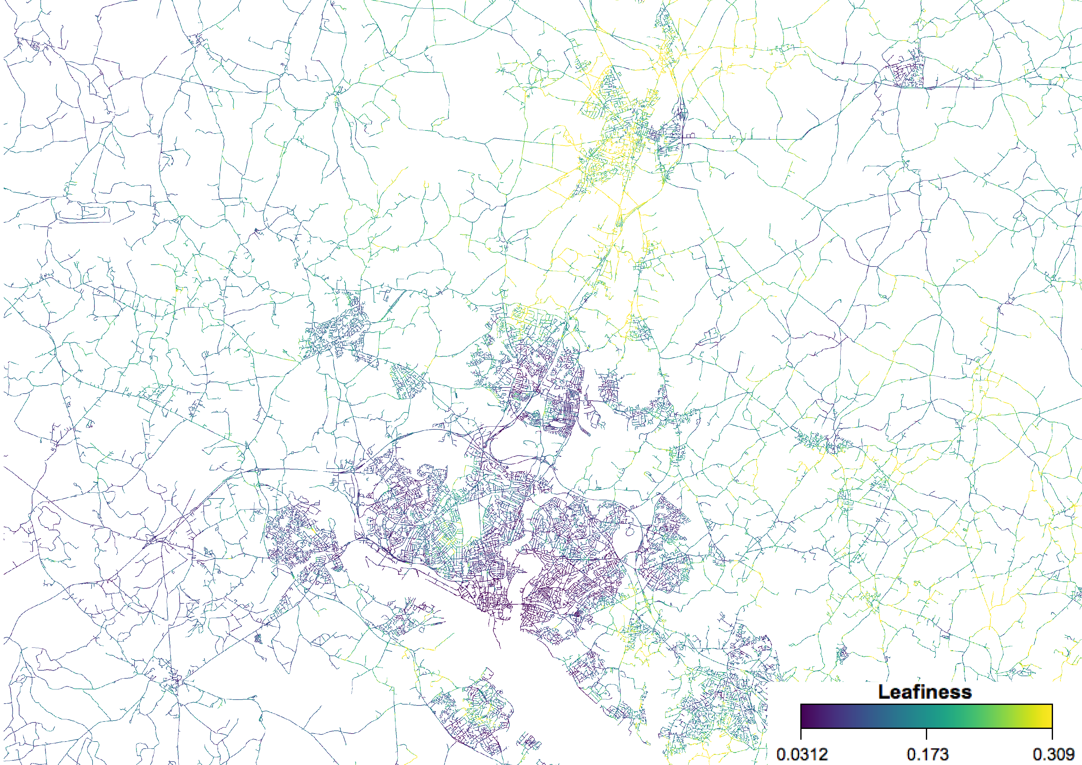
Zooming out to encompass multiple settlements in southern Hampshire, we see a very obvious pattern:
Winchester is completely dominating the area, with far higher values even than most rural areas. Again, this matches up with expectations given that Winchester is a wealthy city, and is known as a nice, leafy place to live. The rural area between Eastleigh and Winchester is also very high, as is – slightly surprisingly – the area around Bursledon to the east of Southampton.
Zooming in on Winchester shows the pattern within the city:
There is a significant east-west divide, with the estates of detached houses that have grown up on the west of the city having very high leafiness, and the older terraced and semi-detached areas on the east of the city having a far lower leafiness.
So, there are some interesting patterns here and some pretty maps. In Part 2, I’ll look at some statistical analysis of leafiness across the England, Wales and Scotland, and then consider some of the limitations of this approach.
I haven’t posted anything on this blog for a long time – sorry about that. I’ve been quite ill, and had a new baby – so blogging hasn’t been my top priority. Hopefully I’ll manage some slightly more regular posts now. Anyway, on with the post…
I recently needed to delete some attribute columns from a very large (multi-GB) shapefile. I had the shapefile open in QGIS, so decided the easiest way would be to do it through the GUI as follows:
Open up the attribute table
Turn on editing (far left toolbar button)
Click the Delete Field button (third from the right, or press Ctrl-L) and select the fields to delete
I was surprised to find that this took ages. It seemed to refresh the attribute table multiple times throughout the process (maybe after deleting each separate field?), and that took ages to do (because the shapefile was so large).
I then found I needed to do this process again, and looked for a more efficient way – and I found one. Unsurprisingly, it uses the GDAL/OGR command-line tools – a very helpful set of tools which often provide superior features and/or performance.
Basically, rather than deleting fields, copy the data to a new file, selecting just the fields that you want. For example:
This will select just the columns attribute1 and attribute2 from the file input.shp.
Surprisingly this command doesn’t actually produce a full shapefile as an output – instead of producing output.shp, output.shx, output.prj and output.dbf (the full set of files that constitute a ‘shapefile’), it just creates output.dbf – the file that contains the attribute table. However, this is easily fixed: just copy the other input.* files and rename them as appropriate (or, if you don’t want to keep the input data, then just rename output.dbf as input.dbf).
I remember experimenting with doing regressions in Python using R-style formulae a long time ago, and I remember it being a bit complicated. Luckily it’s become really easy now – and I’ll show you just how easy.
Before running this you will need to install the pandas, statsmodels and patsy packages. If you’re using conda you should be able to do this by running the following from the terminal:
You may have noticed from the code above that you can just give a URL to the read_csv function and it will download it and open it – handy!
Anyway, here is the data:
df.head()
Model
MPG
Cylinders
Engine Disp
Horsepower
Weight
Accelerate
Year
Origin
0
amc ambassador dpl
15.0
8
390.0
190
3850
8.5
70
American
1
amc gremlin
21.0
6
199.0
90
2648
15.0
70
American
2
amc hornet
18.0
6
199.0
97
2774
15.5
70
American
3
amc rebel sst
16.0
8
304.0
150
3433
12.0
70
American
4
buick estate wagon (sw)
14.0
8
455.0
225
3086
10.0
70
American
Before we do our regression it might be a good idea to look at simple correlations between columns. We can get the correlations between each pair of columns using the corr() method:
df.corr()
MPG
Cylinders
Engine Disp
Horsepower
Weight
Accelerate
Year
MPG
1.000000
-0.777618
-0.805127
-0.778427
-0.832244
0.423329
0.580541
Cylinders
-0.777618
1.000000
0.950823
0.842983
0.897527
-0.504683
-0.345647
Engine Disp
-0.805127
0.950823
1.000000
0.897257
0.932994
-0.543800
-0.369855
Horsepower
-0.778427
0.842983
0.897257
1.000000
0.864538
-0.689196
-0.416361
Weight
-0.832244
0.897527
0.932994
0.864538
1.000000
-0.416839
-0.309120
Accelerate
0.423329
-0.504683
-0.543800
-0.689196
-0.416839
1.000000
0.290316
Year
0.580541
-0.345647
-0.369855
-0.416361
-0.309120
0.290316
1.000000
Now we can do some regression using R-style formulae. In this case we’re trying to predict MPG based on the year that the car was released:
The ‘formula’ that we used above is the same as R uses: on the left is the dependent variable, on the right is the independent variable. The ols method is nice and easy, we just give it the formula, and then the DataFrame to use to get the data from (in this case, it’s called df). We then call fit() to actually do the regression.
We can easily get a summary of the results here – including all sorts of crazy statistical measures!
results.summary()
OLS Regression Results
Dep. Variable:
MPG
R-squared:
0.337
Model:
OLS
Adj. R-squared:
0.335
Method:
Least Squares
F-statistic:
198.3
Date:
Sat, 20 Aug 2016
Prob (F-statistic):
1.08e-36
Time:
10:42:17
Log-Likelihood:
-1280.6
No. Observations:
392
AIC:
2565.
Df Residuals:
390
BIC:
2573.
Df Model:
1
Covariance Type:
nonrobust
coef
std err
t
P>|t|
[95.0% Conf. Int.]
Intercept
-70.0117
6.645
-10.536
0.000
-83.076 -56.947
Year
1.2300
0.087
14.080
0.000
1.058 1.402
Omnibus:
21.407
Durbin-Watson:
1.121
Prob(Omnibus):
0.000
Jarque-Bera (JB):
15.843
Skew:
0.387
Prob(JB):
0.000363
Kurtosis:
2.391
Cond. No.
1.57e+03
We can do a more complex model easily too. First lets list the columns of the data to remind us what variables we have:
We can now add in more variables – doing multiple regression:
model=ols("MPG ~ Year + Weight + Horsepower",data=df)results=model.fit()results.summary()
OLS Regression Results
Dep. Variable:
MPG
R-squared:
0.808
Model:
OLS
Adj. R-squared:
0.807
Method:
Least Squares
F-statistic:
545.4
Date:
Sat, 20 Aug 2016
Prob (F-statistic):
9.37e-139
Time:
10:42:17
Log-Likelihood:
-1037.4
No. Observations:
392
AIC:
2083.
Df Residuals:
388
BIC:
2099.
Df Model:
3
Covariance Type:
nonrobust
coef
std err
t
P>|t|
[95.0% Conf. Int.]
Intercept
-13.7194
4.182
-3.281
0.001
-21.941 -5.498
Year
0.7487
0.052
14.365
0.000
0.646 0.851
Weight
-0.0064
0.000
-15.768
0.000
-0.007 -0.006
Horsepower
-0.0050
0.009
-0.530
0.597
-0.024 0.014
Omnibus:
41.952
Durbin-Watson:
1.423
Prob(Omnibus):
0.000
Jarque-Bera (JB):
69.490
Skew:
0.671
Prob(JB):
8.14e-16
Kurtosis:
4.566
Cond. No.
7.48e+04
We can see that bringing in some extra variables has increased the $R^2$ value from ~0.3 to ~0.8 – although we can see that the P value for the Horsepower is very high. If we remove Horsepower from the regression then it barely changes the results:
model=ols("MPG ~ Year + Weight",data=df)results=model.fit()results.summary()
OLS Regression Results
Dep. Variable:
MPG
R-squared:
0.808
Model:
OLS
Adj. R-squared:
0.807
Method:
Least Squares
F-statistic:
819.5
Date:
Sat, 20 Aug 2016
Prob (F-statistic):
3.33e-140
Time:
10:42:17
Log-Likelihood:
-1037.6
No. Observations:
392
AIC:
2081.
Df Residuals:
389
BIC:
2093.
Df Model:
2
Covariance Type:
nonrobust
coef
std err
t
P>|t|
[95.0% Conf. Int.]
Intercept
-14.3473
4.007
-3.581
0.000
-22.224 -6.470
Year
0.7573
0.049
15.308
0.000
0.660 0.855
Weight
-0.0066
0.000
-30.911
0.000
-0.007 -0.006
Omnibus:
42.504
Durbin-Watson:
1.425
Prob(Omnibus):
0.000
Jarque-Bera (JB):
71.997
Skew:
0.670
Prob(JB):
2.32e-16
Kurtosis:
4.616
Cond. No.
7.17e+04
We can also see if introducing categorical variables helps with the regression. In this case, we only have one categorical variable, called Origin. Patsy automatically treats strings as categorical variables, so we don’t have to do anything special – but if needed we could wrap the variable name in C() to force it to be a categorical variable.
model=ols("MPG ~ Year + Origin",data=df)results=model.fit()results.summary()
OLS Regression Results
Dep. Variable:
MPG
R-squared:
0.579
Model:
OLS
Adj. R-squared:
0.576
Method:
Least Squares
F-statistic:
178.0
Date:
Sat, 20 Aug 2016
Prob (F-statistic):
1.42e-72
Time:
10:42:17
Log-Likelihood:
-1191.5
No. Observations:
392
AIC:
2391.
Df Residuals:
388
BIC:
2407.
Df Model:
3
Covariance Type:
nonrobust
coef
std err
t
P>|t|
[95.0% Conf. Int.]
Intercept
-61.2643
5.393
-11.360
0.000
-71.868 -50.661
Origin[T.European]
7.4784
0.697
10.734
0.000
6.109 8.848
Origin[T.Japanese]
8.4262
0.671
12.564
0.000
7.108 9.745
Year
1.0755
0.071
15.102
0.000
0.935 1.216
Omnibus:
10.231
Durbin-Watson:
1.656
Prob(Omnibus):
0.006
Jarque-Bera (JB):
10.589
Skew:
0.402
Prob(JB):
0.00502
Kurtosis:
2.980
Cond. No.
1.60e+03
You can see here that Patsy has automatically created extra variables for Origin: in this case, European and Japanese, with the ‘default’ being American. You can configure how this is done very easily – see here.
Just for reference, you can easily get any of the statistical outputs as attributes on the results object:
results.rsquared
0.57919459237581172
results.params
Intercept            -61.264305
Origin[T.European]     7.478449
Origin[T.Japanese]     8.426227
Year                   1.075484
dtype: float64
You can also really easily use the model to predict based on values you’ve got:
This is just a very brief reminder about something you might run into when you’re trying to get your code to work on multiple platforms – in this case, OS X, Linux and Windows.
Basically: file names/paths are case-sensitive on Linux, but not on OS X or Windows.
Therefore, you could have some Python code like this:
f = open(os.path.join(base_path, 'LE72020252003106EDC00_B1.tif'))
which you might use to open part of a Landsat 7 image – and it would work absolutely fine on OS X and Windows, but fail on Linux. I initially assumed that the failure on Linux was due to some of the crazy path manipulation stuff that I had done to get base_path – but it wasn’t.
It was purely down to the fact that the file was actually called LE72020252003106EDC00_B1.TIF, and Linux treats LE72020252003106EDC00_B1.tif and LE72020252003106EDC00_B1.TIF as different files.
I’d always known that paths on Windows are not case-sensitive, and that they are case-sensitive on Linux – but I’d naively assumed that OS X paths were case-sensitive too, as OS X is based on a *nix backend, but I was wrong.
If you really have problems with this then you could fairly easily write a function that checked to see if a filename exists, and if it found that it didn’t then tried searching for files using something like a case-insensitive regular expression – but it’s probably just easiest to get the case of the filename right in the first place!
This is a quick post to brief describe a problem I ran into the other day when trying to debug someone’s code – the answer may be entirely obvious to you, but it took me a while to work out, so I thought I’d document it here.
The problem that I was called over to help with was a line of code like this:
t.do_something(a=5, b=10)
where t was an instance of a class. Now, this wasn’t the way that I usually write code – I tend to only use keyword arguments after I’ve already used positional arguments – but it reminded me that in Python the following calls to the function f(a, b) are equivalent:
f(1, 2)
f(1, b=2)
f(a=1, b=2)
Anyway, going back to the original code: it gave the following error:
do_something() got multiple values for argument 'a'
which I thought was very strange, as there was definitely only one value of a given in the call to that method.
If you consider yourself to be a reasonably advanced Python programmer than you might want to stop here and see if you can work out what the problem is. Any ideas?
When you’ve had a bit of a think, continue below…
I had a look at the definition of t.do_something(), and it looked like this:
class Test:

    def do_something(a, b):
        # Do something here!
        print('a = %s' % a)
        print('b = %s' % b)
You may have noticed the problem now – although at first glance I couldn’t see anything wrong… There was definitely only one parameter called a, and it definitely wasn’t being passed twice…so what was going on?!
As you’ve probably noticed by now…this method was missing the self parameter – and should have been defined as do_something(self, a, b). Changing it to that made it work fine, but it’s worth thinking about exactly why we were getting that specific error.
Firstly, let’s have a look at a more ‘standard’ error that you might get when you forget to add self as the first argument for an instance method. We can see this by just calling the method without using keyword arguments (that is, t.do_something(1, 2)), which gives:
TypeError: test_noself() takes 2 positional arguments but 3 were given
Now, once you’ve been programming Python for a while you’ll be fairly familiar with this error from when you’ve forgotten to put self as the first parameter for an instance method. The reason this specific error is produced is that Python will always pass instance methods the value of selfas well as the arguments you’ve given the method. So, when you run the code:
t.do_something(1, 2)
Python will change this ‘behind the scenes’, and actually run:
t.do_something(t, 1, 2)
and as do_something is only defined to take two arguments, you’ll get an error. Of course, if your function had been able to take three arguments (for example, if there was an optional third argument), then you would find that t (which is the value of self in this case) was being passed as the first argument (a), 1 as the value of the second argument (b) and 2 as the value of the third argument (which could have been called c). This is a good point to remind you that the first argument of methods is only called self by convention – and that Python itself doesn’t care what you call it (although you should always call it self!)
From this, you should be able to work out why you’re getting an error about getting multiple values for the argument a… What’s happening is that Python is passing self to the method, as the first argument (which we have called a), and is then passing the two other arguments that we specified as keyword arguments. So, the ‘behind the scenes’ code calling the function is:
t.do_something(t, a=1, b=2)
But, the first argument is called a, so this is basically equivalent to writing:
t.do_something(a=t, a=1, b=2)
which is obviously ambiguous – and so Python throws an error.
Interestingly, it is quite difficult to get into a situation in which Python throws this particular error – if you try to run the code above you get a different error:
SyntaxError: keyword argument repeated
as Python has realised that there is a problem from the syntax, before it even tries to run it. You can manage it by using dictionary unpacking:
def f(a, b):
    pass

d = {'a':1, 'b':2}
f(1, **d)
Here we are defining a function that takes two arguments, and then calling it with a single positional argument for a, and then using the ** method of dictionary unpacking to take the dictionary d and convert each key-value pair to a keyword argument and value combination.
So, congratulations if you’d have solved this problem far quicker than me – but I hope it has made you think a bit more about how Python handles positional and keyword arguments. A few points to remember:
Always remember to use self as the first argument of your methods! (This would have stopped this problem ever happening!)
But remember that the name self is just a convention, and Python will pass the instance of your class to your first argument regardless what it is called, which can cause weird problems.
All positional arguments can be passed as keyword arguments, and vice-versa – they are entirely interchangeable – which, again, can cause problems if this isn’t what you intended.
A key – but challenging – part of learning to program is moving from writing technically-correct code ‘that works’ to writing high-quality code that is sensibly decomposed into functions, generically-applicable and generally ‘good’. Indeed, you could say that this is exactly what Software Carpentry is about – taking you from someone bodging together a few bits of wood in the shed, to a skilled carpenter. As well as being challenging to learn, this is also challenging to teach: how should you show the progression from ‘working’ to ‘good’ code in a teaching context?
I’ve been struggling with this recently as part of some small-group programming teaching I’ve been doing. Simply showing the ‘before’ and ‘after’ ends up bombarding the students with too many changes at once: they can’t see how you get from one to the other, so I want some way to show the development of code over time as things are gradually done to it (for example, moving this code into a separate function, adding an extra argument to that function to make it more generic, renaming these variables and so on). Obviously when teaching face-to-face I can go through this interactively with the students – but some changes to real-world code are too large to do live – and students often seem to find these sorts of discussions a bit overwhelming, and want to refer back to the changes and reasoning later (or they may want to look at other examples I’ve given them). Therefore, I want some way to annotate these changes to give the explanation (to show why we’re moving that bit of code into a separate function, but not some other bit of code), but to still show them in context.
Exactly what code should be used for these examples is another discussion: I’ve used real-world code from other projects, code I’ve written specifically for demonstration, code I’ve written myself in the past and sometimes code that the students themselves have written.
So far, I’ve tried the following approaches for showing these changes with annotation:
Making all of the changes to the code and providing a separate document with an ordered list of what I’ve changed and why. Simple and low-tech, but often difficult for the students to visualise each change
The same as above but committing between each entry in the list. Allows them to step through git commits if they want, and to get back to how the code was after each individual change – but many of the students struggle to do this effectively in git, and it adds a huge technological barrier – particularly with Git’s ‘interesting’ user-interface.
The same as above, but using Github’s line comments feature to put comments at specific locations in the code. Allows annotations at specific locations in the code, but rather clunky to step through the full diff view of commits in order using Github’s UI.
I suspect any solution will involve some sort of version control system used in some way (although I’m not sure that standard diffs are quite the best way to represent changes for this particular use-case), but possibly with a different interface on it.
Is this a problem anyone else has faced in their teaching? Can you suggest any tools or approaches that might make this easier – for both the teacher and students?
I use data from the AERONET network of sun photometers a lot in my work, and do a lot of processing of the data in Python. As part of this I usually want to load the data into pandas – but because of the format of the data, it’s not quite as simple as it could be.
So, for those of you who are impatient, here is some code that reads an AERONET data file into a pandas DataFrame which you can just download and use:
For those who want more details, read on…
Once you’ve downloaded an AERONET data file and unzipped it, you’ll find you have a file called something like 050101_161231_Chilbolton.lev20, and if you look at the start of the file it’ll look a bit like this:
Level 2.0. Quality Assured Data.<p>The following data are pre and post field calibrated, automatically cloud cleared and manually inspected.
Version 2 Direct Sun Algorithm
Location=Chilbolton,long=-1.437,lat=51.144,elev=88,Nmeas=13,PI=Iain_H._Woodhouse_and_Judith_Agnew_and_Judith_Jeffrey_and_Judith_Jeffery,Email=fsf@nerc.ac.uk_and__and__and_judith.jeffery@stfc.ac.uk
AOD Level 2.0,All Points,UNITS can be found at,,, http://aeronet.gsfc.nasa.gov/data_menu.html
Date(dd-mm-yy),Time(hh:mm:ss),Julian_Day,AOT_1640,AOT_1020,AOT_870,AOT_675,AOT_667,AOT_555,AOT_551,AOT_532,AOT_531,AOT_500,AOT_490,AOT_443,AOT_440,AOT_412,AOT_380,AOT_340,Water(cm),%TripletVar_1640,%TripletVar_1020,%TripletVar_870,%TripletVar_675,%TripletVar_667,%TripletVar_555,%TripletVar_551,%TripletVar_532,%TripletVar_531,%TripletVar_500,%TripletVar_490,%TripletVar_443,%TripletVar_440,%TripletVar_412,%TripletVar_380,%TripletVar_340,%WaterError,440-870Angstrom,380-500Angstrom,440-675Angstrom,500-870Angstrom,340-440Angstrom,440-675Angstrom(Polar),Last_Processing_Date(dd/mm/yyyy),Solar_Zenith_Angle
10:10:2005,12:38:46,283.526921,N/A,0.079535,0.090636,0.143492,N/A,N/A,N/A,N/A,N/A,0.246959,N/A,N/A,0.301443,N/A,0.373063,0.430350,2.115728,N/A,0.043632,0.049923,0.089966,N/A,N/A,N/A,N/A,N/A,0.116690,N/A,N/A,0.196419,N/A,0.181772,0.532137,N/A,1.776185,1.495202,1.757222,1.808187,1.368259,N/A,17/10/2006,58.758553
You can see here that we have a few lines of metadata at the top of the file, including the ‘level’ of the data (AERONET data is provided at three levels, 1.0, 1.5 and 2.0, referring to the quality assurance of the data), and some information about the AERONET site.
In this function we’re just going to ignore this metadata, and start reading at the 5th line, which contains the column headers. Now, you’ll see that the data looks like a fairly standard CSV file, so we should be able to read it fairly easily with pd.read_csv. This is true, and you can read it using:
df = pd.read_csv(filename, skiprows=4)
However, you’ll find a few issues with the DataFrame you get back from that simple line of code: firstly dates and times are just left as strings (rather than being parsed into proper datetime columns) and missing data is still shown as the string ‘N/A’. We can solve both of these:
No data: read_csv allows us to specify how ‘no data’ values are represented in the data, so all we need to do is set this: pd.read_csv(filename, skiprows=4, na_values=['N/A']) Note: we need to give na_values a list of values to treat as no data, hence we create a single-element list containing the string N/A.
Dates & times: These are a little harder, mainly because of the strange format in which they are provided in the file. Although the column header for the first column says Date(dd-mm-yy), the date is actually colon-separated (dd:mm:yy). This is a very unusual format for a date, so pandas won’t automatically convert it – we have to help it along a bit. So, first we define a function to parse a date from that strange format into a standard Python datetime:
I could have written this as a normal function (def dateparse(x)), but I used a lambda expression as it seemed easier for such a short function. Once we’ve defined this function we tell pandas to use it to parse dates (date_parser=dateparse) and also tell it that the first two columns together represent the time of each observation, and they should be parsed as dates (parse_dates={'times':[0,1]}).
That’s all we need to do to read in the data and convert the right columns, the rest of the function just does some cleaning up:
We set the times as the index of the DataFrame, as it is the unique identifier for each observation – and makes it easy to join with other data later.
We remove the JulianDay column, as it’s rather useless now that we have a properly parsed timestamp
We drop any columns that are entirely NaN and any rows that are entirely NaN (that’s what dropna(axis=1, how='all') does).
We rename a column, and then make sure the data is sorted
aeronet = aeronet.set_index('times')
del aeronet['Julian_Day']

# Drop any rows that are all NaN and any cols that are all NaN
# & then sort by the index
an = (aeronet.dropna(axis=1, how='all')
            .dropna(axis=0, how='all')
            .rename(columns={'Last_Processing_Date(dd/mm/yyyy)': 'Last_Processing_Date'})
            .sort_index())
You’ll notice that the last few bits of this ‘post-processing’ were done using ‘method-chaining’, where we just ‘chain’ pandas methods one after another. This is often a very convenient way to work in Python – see this blog post for more information.
So, that’s how this function works – now go off and process some AERONET data!
I now use Anaconda as my primary Python distribution – and my company have also adopted it for use on all of their developer machines as well as their servers – so I like to think I’m a relatively knowledgeable user. However, the other day I came across a wonderful feature that I’d never known about before…revisions!
The best way to explain is by a quick example. If you run conda list --revisions, you’ll get an output like this:
In this output you can see a number of specific versions (or revisions) of this environment (in this case the default conda environment), along with the date/time they were created, and the differences (installed packages shown as +, uninstalled shown as - and upgrades shown as ->). If you want to revert to a previous revision you can simply run conda install --revision N (where N is the revision number). This will ask you to confirm the relevant package uninstallation/installation – and get you back to exactly where you were before!
So, I think that’s pretty awesome – and really handy if you screw things up and want to go back to a previously working environment. I’ve got a few other hints for you though…
Firstly, if you ‘revert’ to a previous revision then you will find that an ‘inverse’ revision is created, simply doing the opposite of what the previous revision did. For example, if your revision list looks like this:
You can see that the changes for revision 3 are just the inverse of revision 2.
One more thing is that I’ve found out that all of this data is stored in the history file in the conda-meta directory of your environment (CONDA_ROOT/conda-meta for your default environment and CONDA_ROOT/envs/ENV_NAME/conda-meta for any other environment). You don’t want to know why I went searching for this file (it’s a long story involving some stupidity on my part), but it’s got some really useful contents:
Specifically, it doesn’t just give you the list of what was installed, uninstalled or upgraded – but it also gives you the commands you ran! If you want, you can extract these commands with a bit of command-line magic:
(For reference, the command-line magic gets the content of the history file, searches for all lines starting with # cmd, and then splits the line by spaces and extracts everything from the 3rd group onwards)
I find environment.yml files to be a bit of a pain sometimes (they’re not always cross-platform compatible – see this issue), so this is quite useful as it actually gives me the commands that I ran to create the environment.
There was a question recently on the Py6S mailing list about what data sources are best to use to provide atmospheric parameters (such as AOT, water vapour and ozone) for use with 6S, other atmospheric Radiative Transfer Models (such as MODTRAN) or other atmospheric correction algorithms (such as ATCOR). In the spirit of ‘reply to public’ I decided I’d post the response here, as it’d certainly be easier for other people to find in future!
The first thing to say is if you’re doing atmospheric correction, then by far the best solution is to derive as many of the parameters as possible from the satellite data that you are trying to correct. Sometimes this is relatively easy (for example, when using MODIS data, as there are standard MODIS products for AOT, water vapour and ozone) and sometimes harder (there are no standard atmospheric products for SPOT, and algorithms for estimating atmospheric parameters from Landsat are relatively limited). The main reasons for this are:
The atmospheric data will be from the exact time of the satellite image acquisition
Depending on the satellite, the atmospheric data may be provided for every pixel in the image, and if this isn’t the case then there might be more than one value across the image (for example, the LEDAPS algorithm estimates AOT over all pixels containing Dense Dark Vegetation). This is key as it allows the atmospheric correction algorithm to take into account changes in atmospheric conditions across the image. I have published research (Wilson et al., 2014) showing that failing to take into account this variability when doing atmospheric correction can lead to significant errors.
However, if you’ve found this post then you’ve probably either already tried using data from the satellite you’re working with, and found it isn’t possible – or you’re doing radiative transfer modelling for some other purpose than atmospheric correction, so the explanation above had no relevance to you. So, on with the other data sources – and in Part 1 we’re going to cover aerosol-related data.
Aerosol Optical Thickness
(Also known as Aerosol Optical Depth, just to confuse you!)
This is a measure of the haziness of the atmosphere, and is set in Py6S as: s.aot550 = x Please note that this means AOT at 550nm (yes, AOT is wavelength dependent!), so you may have to interpolate the AOT data from different wavelengths. I’ll post a separate post soon about how best to do this.
When choosing an AOT data source, you usually have a trade-off between accuracy, spatial resolution and temporal resolution. If you’re lucky, you can manage to get two of those, but not three! So, going in order of accuracy:
AERONET
The Aerosol Robotic Network (AERONET) is the gold-standard in terms of accurate measurement of AOT. The measurements are acquired from ground-based sun photometers, which have the major benefit of being able to produce very accurate measurements at a high frequency – as they don’t depend on satellite orbits. However, there are two major disadvantages: they have a very low spatial resolution, and they only produce measurements when the sun is shining.
Specifically, although there are over 1,000 measurement sites listed on the AERONET website, many of these are for short-term measurement campaigns and so the number of sites regularly recording measurements over a long period of time is much lower. For example, excluding short-term sites, there are only three measurement sites in the UK (Hampshire, London and Edinburgh), and there are many parts of the world with very few sites (such as central Africa).
Also, as mentioned above, measurements are only acquired when there is a direct view of the sun from the instrument. This obviously means that measurements are not acquired during the night (which can stretch for many months near the poles), but also that cloud cover has a significant impact on the frequency of measurements. The AERONET cloud-screening algorithms have to be very strict, as even a tiny amount of cloud will cause a large error in the AOT measurement.
Good for: Very accurate measurements. High temporal resolution.
Bad for: Spatially-dense measurements. Cloudy areas.
AERONET run a large network of sun photometers, but there are many other sun photometers run by other people/groups, and these can be good sources of data. Indeed, you may even have acquired your own measurements using your own sun photometer (such as the Microtops sun photometer pictured below). The advantages and disadvantages above still apply, although if you’ve taken measurements yourself then I assume they are in the right place and at the right time!
Data available from: There is a (slightly old now) list of other sun photometer data sources online. If you’ve got Microtops data that you want to process then have a look at my PyMicrotops module that makes the process a lot easier.
MODIS AOT
Data from the MODIS sensor on the Aqua and Terra satellites is operationally processed to produce AOT data at 10km and 3km resolution, the MOD04 and MOD04_3K products. AOT estimates are produced over all land surfaces, but measurements over bright surfaces (such as deserts and snow) tend to have a higher error.
The Aqua and Terra satellites are in a sun-synchronous orbit, so passes over each location at approximately 10:30 and 13:30 local solar time, giving a total of two measurements a day. Again, cloud cover is an issue, and the MODIS algorithm masks out any pixel containing cloud.
The MODIS data is provided as HDF files with loads of Scientific Data Sets (SDS, basically bands) – the one you want to use is called Optical_Depth_Land_And_Ocean, which is high quality AOT data (where the QAC, the measure of retrieval quality, is 3) from both land and ocean, using all algorithms.
The MOD08 dataset provides the same data at a lower resolution (1 degree), if spatial resolution is not important for you.
Good for: Moderate spatial resolution. Operational data availability. Reasonable accuracy.
Bad for: Temporal resolution. Cloudy areas.
Data available from: LAADSWeb (Unfortunately it comes in an annoying projection, but you can reproject it using the MODIS Reprojection Tool or HEG. MOD08 doesn’t have this issue, and can also be accessed through Google Earth Engine)
MAIAC
The Multi-Angle Implementation of Atmospheric Correction (MAIAC) algorithm (Lyapustin et al., 2011) produces AOT data at 1km resolution, through a novel method which combines a range of MODIS observations with differing view geometries.
Good for: High spatial resolution.
Bad for: Not currently operationally available.
Data available from: Data is not currently available online, but I think it is due to be released as an official MODIS product within the next six months or so.
Aerosol Type
There are lots of ways of parameterising aerosol types in radiative transfer models (see here for a list of the ways you can do this in Py6S) – and it is often difficult to work out what the best option to use is. I’ve listed some options below, but this is unlikely to be a comprehensive list – so please leave a comment if you know of any other data sources.
AERONET
As well as providing AOT data, AERONET sun photometers also acquire other measurements which can be used to infer the aerosol type. This is almost certainly the most accurate way of setting the aerosol type – and there is a built-in function in Py6S that will help you do it. See here for full details on how to use it: basically you just download the AERONET data and give Py6S the filename and date/time and it does the rest.
Data available from: NASA AERONET site (find AERONET Inversions on the left-hand side)
MODIS
The MOD04 product mentioned above also provides an estimation of aerosol type, in five categories: dust, sulfate, smoke, heavy absorbing smoke and mixed. It’s not entirely clear how best to match these to the predefined 6S aerosol types (which are biomass burning, continental, desert, maritime, stratospheric and urban) – although there is an option in 6S to set a user-defined aerosol profile, which allows you to specify the relative fraction of each of dust, water, oceanic and soot aerosols (see AeroProfile.User)
Data available from: LAADSWeb (Unfortunately it comes in an annoying projection, but you can reproject it using the MODIS Reprojection Tool or HEG.)
Aerosol type climatologies
A number of aerosol type climatologies have been produced, giving an indication of the typical aerosol type observed at each location, over time. These climatologies vary in the level of detail – both in terms of spatial resolution (which is often coarse) and temporal resolution (often monthly or seasonally). The best way to find these is to search for papers about aerosol climatologies, and then either look for a URL in the paper or contact the authors to ask for the data. I’ve only included a couple of examples here as new climatologies are being published frequently:
Clim-Likely: Data available here, at 1 x 1 degree resolution
So, that’s it for this part. Please let me know of any datasets that I’ve missed – and stay tuned for Part 2 which will cover other parameters (water vapour, ozone and so on).