Searching an aerial photo with text queries – a demo and how it works
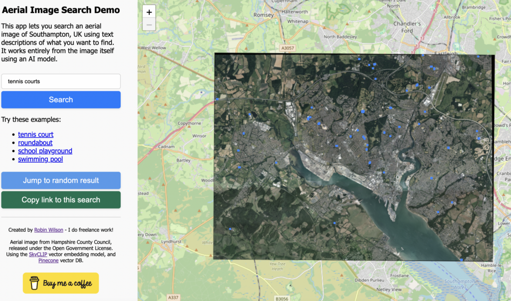
Summary: I’ve created a demo web app where you can search an aerial photo of Southampton, UK using text queries such as "roundabout", "tennis court" or "ship". It uses vector embeddings to do this – which I explain in this blog post.
In this post I’m going to try and explain a bit more about how this works.
Firstly, I should explain that the only data used for the searching is the aerial image data itself – even though a number of these things will be shown on the OpenStreetMap map, none of that data is used, so you can also search for things that wouldn’t be shown on a map (like a blue bus)
The main technique that lets us do this is vector embeddings. I strongly suggest you read Simon Willison’s great article/talk on embeddings but I’ll try and explain here too. An embedding model lets you turn a piece of data (for example, some text, or an image) into a constant-length vector – basically just a sequence of numbers. This vector would look something like [0.283, -0.825, -0.481, 0.153, ...] and would be the same length (often hundreds or even thousands of elements long) regardless how long the data you fed into it was.
In this case, I’m using the SkyCLIP model which produces vectors that are 768 elements long. One of the key features of these vectors are that the model is trained to produce similar vectors for things that are similar in some way. For example, a text embedding model may produce a similar vector for the words "King" and "Queen", or "iPad" and "tablet". The ‘closer’ a vector is to another vector, the more similar the data that produced it.
The SkyCLIP model was trained on image-text pairs – so a load of images that had associated text describing what was in the image. SkyCLIP’s training data "contains 5.2 million remote sensing image-text pairs in total, covering more than 29K distinct semantic tags" – and these semantic tags and the text descriptions of them were generated from OpenStreetMap data.
Once we’ve got the vectors, how do we work out how close vectors are? Well, we can treat the vectors as encoding a point in 768-dimensional space. That’s a bit difficult to visualise – so imagine a point in 2- or 3-dimensional space as that’s easier, plotted on a graph. Vectors for similar things will be located physically closer on the graph – and one way of calculating similarity between two vectors is just to measure the multi-dimensional distance on a graph. In this situation we’re actually using cosine similarity, which gives a number between -1 and +1 representing the similarity of two vectors.
So, we now have a way to calculate an embedding vector for any piece of data. The next step we take is to split the aerial image into lots of little chunks – we call them ‘image chips’ – and calculate the embedding of each of those chunks, and then compare them to the embedding calculated from the text query.
I used the RasterVision library for this, and I’ll show you a bit of the code. First, we generate a sliding window dataset, which will allow us to then iterate over image chips. We define the size of the image chip to be 200×200 pixels, with a ‘stride’ of 100 pixels which means each image chip will overlap the ones on each side by 100 pixels. We then configure it to resize the output to 224×224 pixels, which is the size that the SkyCLIP model expects as input.
ds = SemanticSegmentationSlidingWindowGeoDataset.from_uris(
        image_uri=uri,
        image_raster_source_kw=dict(channel_order=[0, 1, 2]),
        size=200,
        stride=100,
        out_size=224,
    )
We then iterate over all of the image chips, run the model to calculate the embedding and stick it into a big array:
dl = DataLoader(ds, batch_size=24)

EMBEDDING_DIM_SIZE = 768
embs = torch.zeros(len(ds), EMBEDDING_DIM_SIZE)

with torch.inference_mode(), tqdm(dl, desc='Creating chip embeddings') as bar:
    i = 0
    for x, _ in bar:
        x = x.to(DEVICE)
        emb = model.encode_image(x)
        embs[i:i + len(x)] = emb.cpu()
        i += len(x)

# normalize the embeddings
embs /= embs.norm(dim=-1, keepdim=True)

embs.shape
We also do a fair amount of fiddling around to get the locations of each chip and store those too.
Once we’ve stored all of those (I’ll get on to storage in a moment), we need to calculate the embedding of the text query too – which can be done with code like this:
text = tokenizer(text_queries)
with torch.inference_mode():
        text_features = model.encode_text(text.to(DEVICE))
        text_features /= text_features.norm(dim=-1, keepdim=True)
        text_features = text_features.cpu()
It’s then ‘just’ a matter of comparing the text query embedding to the embeddings of all of the image chips, and finding the ones that are closest to each other.
To do this, we can use a vector database. There are loads of different vector databases to choose from, but I’d recently been to a tutorial at PyData Southampton (I’m one of the co-organisers, and I strongly recommend attending if you’re in the area) which used the Pinecone serverless vector database, and they have a fairly generous free tier, so I thought I’d try that.
Pinecone, like all other vector databases, allows you to insert a load of vectors and their metadata (in this case, their location in the image) into the database, and then search the database to find the vectors closest to a ‘search vector’ you provide.
I won’t bother showing you all the code for this side of things: it’s fairly standard code for calling Pinecone APIs, mostly copied from their tutorials.
I then wrapped this all up in a FastAPI API, and put a simple Javascript front-end on it to display the results on a Leaflet web map. I also added some basic caching to stop us hitting the Pinecone API too frequently (as there is limit to the number of API calls you can make on the free plan). And that’s pretty-much it.
I hope the explanation made sense: have a play with the app here and post a comment with any questions.
If you found this post useful, please consider buying me a coffee.
This post originally appeared on Robin's Blog.
Categorised as: Academic, GIS, Programming, Python, Remote Sensing
Hello, after reading your blog, I was deeply impressed. I noticed there’s an image geolocation method in current algorithms, but it has limited positioning accuracy for low-resolution images. Would it be possible to combine a semantic localization approach with image-based localization in order to improve overall accuracy? I’ve been researching this topic myself and would like to consult you on a few related issues. If you don’t mind, could you share your source code with me for further study? I would be extremely grateful.
[…] Using a vector database, SkyCLIP, and Leaflet to create a searchable aerial photograph […]