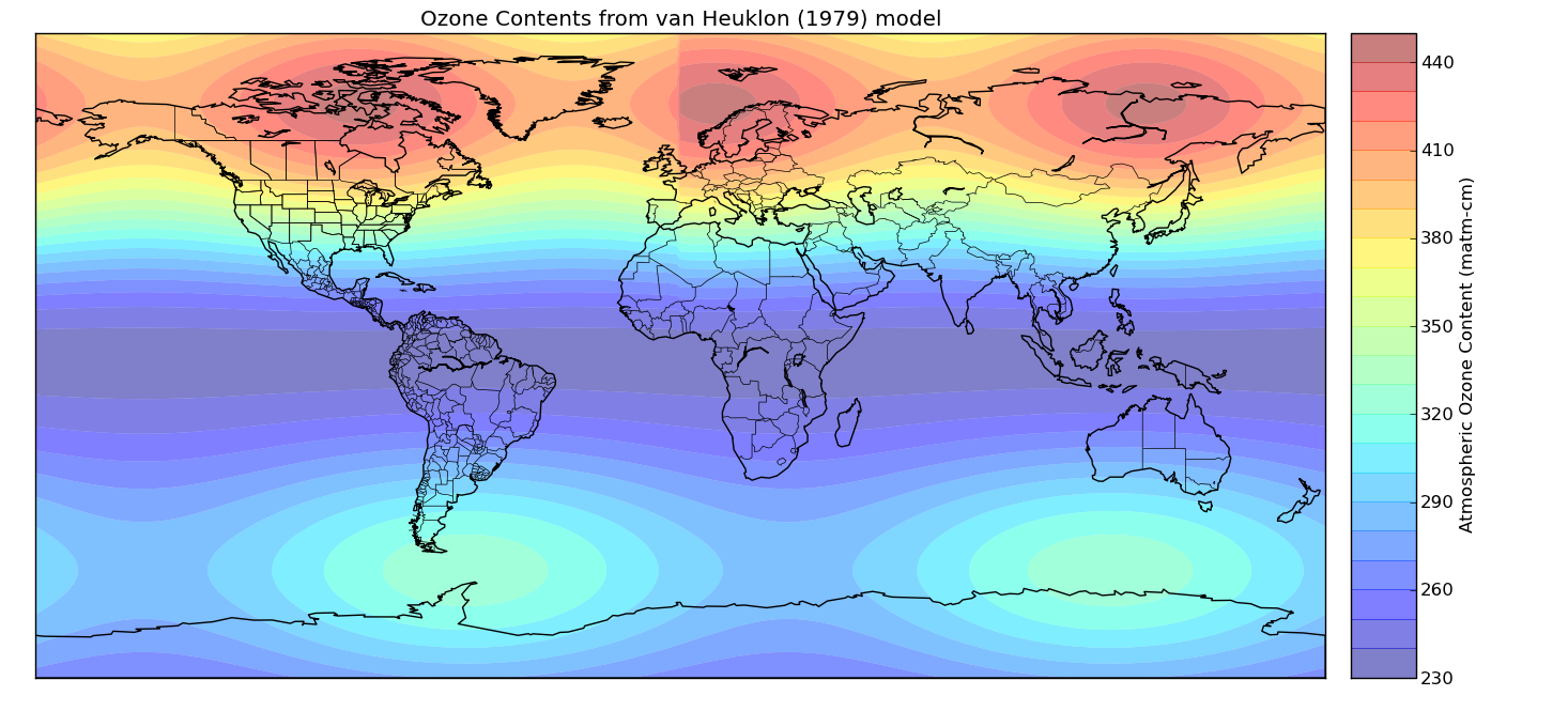
I was going to post this as one of my ‘previously unpublicised code’ posts, but that would be stretching the title a bit, as I have previously blogged about my implementation of the van Heuklon (1979) ozone model.
This is just a brief update (in the spirit of my ‘previously unpublicised code’ posts) to say that I have now packaged up my implementation as a proper python package, added a bit more documentation, and a license and all of the other things that a proper library should have. I can’t say it’s the most exciting library ever – it has one function in it – but it could be useful for someone.
So, next time you need to calculate ozone concentrations (and, be honest, you know the time will come when you need to do that), just run:
and then you can simply run something like this to get all of the ozone concentration estimates you could ever need:
from vanHOzone import get_ozone_conc
get_ozone_conc(50.3, -1.34, '2015-03-14 13:00')
The full documentation is in the docstring:
get_ozone_conc(lat, lon, timestamp)
Returns the ozone contents in matm-cm for the given latitude/longitude and timestamp (provided as either a datetime object or a string in any sensible format - I strongly recommend using an ISO 8601 format of yyyy-mm-dd) according to van Heuklon's Ozone model.
The model is described in Van Heuklon, T. K. (1979). Estimating atmospheric ozone for solar radiation models. Solar Energy, 22(1), 63-68.
This function uses numpy functions, so you can pass arrays and it will return an array of results. The timestamp argument can be either an array/list or a single value. If it is a single value then this will be used for all lat/lon values given.
(as an aside, this is my first time of releasing a conda package, and I think it worked ok!)
No, I’m not seven years old (even though I may act like it sometimes)…but this blog is! My first blog post was on the 11th November 2008 – a rather philosophical post entitled Wisdom and Knowledge – and so on this anniversary I thought I’d look at my blog over the years, the number of visits I’ve got, my most popular posts, and so on.
The earliest snapshot of my website available at www.archive.org is shown below, with my second ever post on the home page (an article that was later republished in the Headington School magazine).
Traffic
Unfortunately it’s a little difficult to look at statistics across the whole of this blog’s life – as I used to use Piwik for website analytics, but switched to Google Analytics part-way through 2014 (when Piwik just got too slow to use effectively). Cleverly, I didn’t export my Piwik data first – so I can’t look at any statistics prior to 2014.
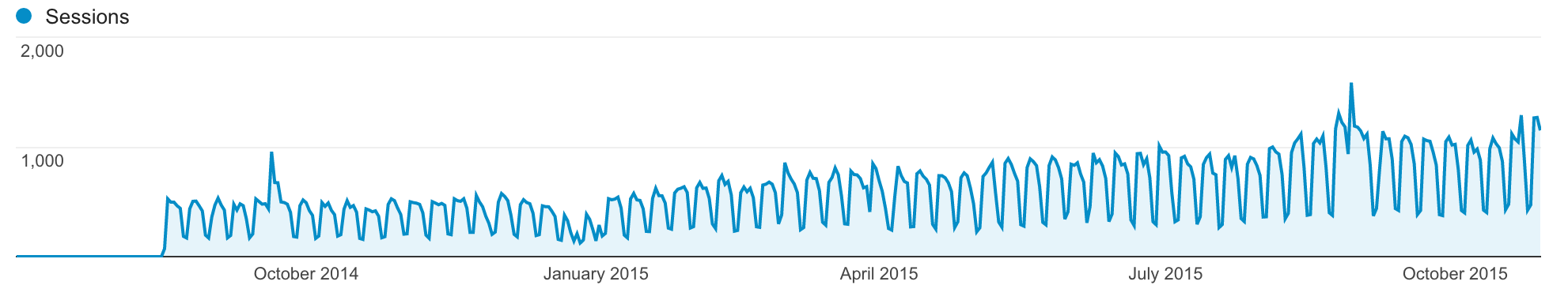
However, I can say that since August 2014, around 240,000 people have viewed my blog, with around 300,000 individual page views – a fairly impressive total, averaging at around 15,000-20,000 visitors per month, but increasing in recent months to around 25,000 per month.
There’s a very noticeable pattern in page views, with significantly fewer views at weekends – probably reflecting the work-like nature of my blog.
The vast majority of these views come from so-called ‘organic searches’ – basically just people searching online for something. The referrals I get tend to be either from social networks (mainly Twitter, but sometimes Facebook too), or from ‘blog aggregators’ that some of my posts are contributed to (my R posts can be found on R Bloggers and my Python posts on Planet Python).
Most popular posts
So, what are these people coming to read? Well, a lot of them are coming to find out how to fix a network printer suddenly showing as offline in Windows – in fact, 51% of all of my page views have been for that post! It’s actually become quite popular – being linked from Microsoft support pages, Microsoft TechNet forums, SpiceWorks forums and more.
My second most popular post is also a how to post – in this case, how to solve Ctrl-Space autocomplete not working in Eclipse (10% of page views), and my third most popular ‘post’ is actually the second page of comments for the network printer post…obviously people are very keen to fix their network printers!
These posts make sense as the most frequently viewed posts: they are either posts that help solve very frustrating problems, posts which have been linked from high-traffic websites (like the Guardian), posts which show you how to do something useful, or posts that have received a lot of attention on Twitter.
My favourite posts
It’s hard to choose some favourites from the 130-odd (some veryodd!) posts that I’ve published – but I’m going to try and choose some from various categories:
Want to write some code? Get away from your computer – I reference this post a lot when teaching programming, as it is far too tempting (particularly for newbies) to start fiddling around with the code, rather than actually thinking!
(These posts had good ideas in them, but I never really followed them up…maybe in the future)
Rules of thumb in remote sensing – a list of common ‘rules of thumb’ in my field and roughly where they come from. I think this sort of ‘common sense’ should be documented more in most fields.
Well, partly because it’s fun, partly because it’s useful and partly because I feel I ought to. Let’s take those separately:
It’s fun to write interesting articles about things. I enjoy sharing my knowledge about topics that I know a lot about, and I enjoy writing the morephilosophicalarticles.
It’s useful because it records information that I tend to forget (I can never remember why I get this error message without looking it up – and I’ve found my own blog from Google searches many times!), it gets me known in the community, it publicises the thingsthatIdo, and it shares useful information with other people.
I feel that I have an obligation to share things, from two perspectives: 1) As a scientist, who is funded mostly by taxpayers, I feel I need to share my researchwork with the public and 2) As a user of lots of open-source software, I feel a need to share someofmycode, and share my knowledgeaboutprogramming.
(For another useful guide on reasons to blog as an academic, see Matt Might’s article – in fact, read his whole blog – it’s great!)
Conclusion
I started this blog as an experiment: I had no idea what I would write, and no idea whether anyone would read it. I posted very little in the first few years, but have been posting semi-regularly since 2011, and people actually seem to be reading it. Hopefully, I will continue for another seven years…
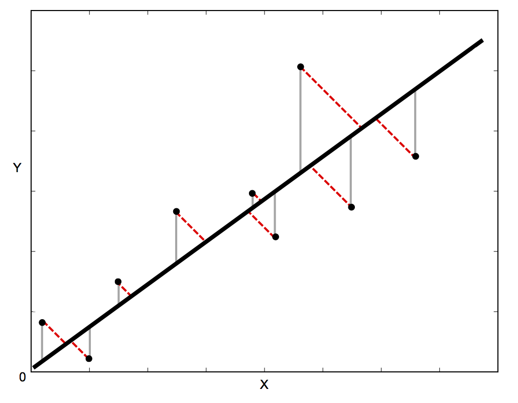
Linear regression is often used to estimate the relationship between two variables – basically by drawing the ‘line of best fit’ on a graph. The mathematical method that is used for this is known as Least Squares, and aims to minimise the sum of the squared error for eachpoint. The key question here is how do you calculate the error (also known as the residual) for each point?
In standard linear regression, the aim is to predict the the Y value from the X value – so the sensible thing to do is to calculate the error in the Y values (shown as the gray lines in the image below). However, sometimes it’s more sensible to take into account the error in both X and Y (as shown by the dotted red lines in the image below) – for example, when you know that your measurements of X are uncertain, or when you don’t want to focus on the errors of one variable over another.
Orthogonal Distance Regression (ODR) is a method that can do this (orthogonal in this context means perpendicular – so it calculates errors perpendicular to the line, rather than just ‘vertically’). Unfortunately, it’s a lot more complicated to implement than standard linear regression, but fortunately there is some lovely Fortran code called ODRPACK that does it for us. Even more fortunately, the lovely scipy people have wrapped this Fortran code in the scipy.odr Python module.
However, because of the complexity of the underlying method, using the scipy.odr module is a lot harder than the simple scipy.stats.linregress function – so I’ve written some code to make it easier. The code below provides a function, orthoregress, which implements ODR and behaves in exactly the same way as the linregress function. For more information, see the ODRPACK User Guide, and the scipy.odr documentation.
When looking through my profile on Github recently, I realised that I had over fifty repositories – and a number of these weren’t really used much by me anymore, but probably contained useful code that no-one really knows about! So, I’m going to write a series of posts giving brief descriptions of the code and what it does, and point people to the Github repository and any documentation (if available). I’m also going make sure that I take this opportunity to ensure that every repository that I publicise has a README file and a LICENSE file.
So, let’s get going with the first repository, which is RTWIDL: a set of useful functions for the IDL programming language. It’s slightly incorrect to call this "unpublicised" code as there has been a page on my website for a while, but it isn’t described in much detail there.
These functions were written during my Summer Bursary at the University of Southampton, and are mainly focused around loading data from file formats that aren’t supported natively by IDL. Specifically, I have written functions to load data from the OceanOptics SpectraSuite software (used to record spectra from instruments like the USB2000), Delta-T logger output files, and NEODC Ames format files. This latter format is interesting – it’s a modification of the NASA Ames file format, so that it can store datetime information as the independent variable. Unfortunately, due to this change none of the ‘standard’ functions for reading NASA Ames format data in IDL will work with this data. Quite a lot of data is available in this format, as for a number of years it was the format of choice of the National Earth Observation Data Centre in the UK (see their documentation on the format). Each of these three functions has detailed documentation, in PDF format, available here.
As well as these functions, there are also a few utility functions for checking whether ENVI is running, loading files into ENVI without ENVI ‘taking over’ the IDL variable, and displaying images with default min-max scaling. These aren’t documented so well, but should be fairly self-explanatory.
NASA image ID AS17-148-22727 is famous. Although you may not recognise the number, you will almost certainly recognise the image:
This was taken by NASA Apollo astronauts on the 7th December 1972, while the Apollo 17 mission was on its way to the moon. It has become one of the most famous photographs ever taken, and has been widely credited as providing an important contribution to the ‘green revolution’, which was rapidly growing in the early 1970s.
It wasn’t, in fact, the first image of the whole Earth to be taken from space – the first images were taken by the ATS-III satellite in 1967, but limitations in satellite imaging at the time meant that their quality was significantly lower:
The Apollo astronauts had the benefit of a high-quality Hasselblad film camera to take their photographs – hence the significantly higher quality.
Part of the reason that this image has become so famous, is because there haven’t been any more like it – Apollo 17 was the last manned lunar mission, and we haven’t sent humans that far away from the Earth since. NASA has released a number of mosaics of satellite images from satellites such as MODIS and Landsat and called these ‘Blue Marble’ images – but they’re not quite the same thing!
Anyway, fast-forwarding to 2015…and NASA launched DSCOVR, the Deep Space Climate Observatory satellite (after a long political battle with climate-change-denying politicians in the United States). Rather than orbiting relatively close to the Earth (around 700km for polar orbiting satellites, and 35,000km for geostationary satellites), DSCOVR sits at the ‘Earth-Sun L1 Lagrangian point’, around 1.5 million km from Earth!
At this distance, it can do a lot of exciting things – such as monitor the solar wind and Coronal Mass Ejections – as it has a continuous view of both the sun and Earth. From our point of view here, the Earth part of this is the most interesting – as it will constantly view the sunny side of the Earth, allowing it to take ‘Blue Marble’ images multiple times a day.
The instrument that acquires these images is called the Earth Polychromatic Imaging Camera (EPIC, hence my little pun in the title), and it takes many sequential Blue Marble images every day. At least a dozen of these images each day are made available on the DSCOVR:EPIC website – within 36 hours of being taken. As well as providing beautiful images (with multiple images per day meaning that it’s almost certain that one of the images will cover the part of the Earth where you live!), EPIC can also be used for proper remote-sensing science – allowing scientists to monitor vegetation health, aerosol effects and more at a very broad spatial scale (but with a very high frequently).
So, in forty years we have moved from a single photograph, taken by a human risking his life around 45,000km from Earth, to multiple daily photographs taken by a satellite orbiting at 1.5 million km from Earth – and providing useful scientific data at the same time (other instruments on DSCOVR will provide warnings of ‘solar storms’ to allow systems on Earth to be protected before the ‘storm’ arrives – but that’s not my area of expertise).
So, click this link and go and look at what the Earth looked like yesterday, from 1.5 million km away, and marvel at the beautiful planet we live on.
I bought a new laptop recently, and just realised that I hadn’t installed two great IPython extensions that I always try to install whenever I set up a new IPython environment – so I thought I’d blog about them to let the world (well, my half-a-dozen readers) know.
They’re both written by MinRK – one of the core IPython developers – and provide some really useful additional functionality. If you’re impatient, then download them here, otherwise read on to find out what they do.
Table of Contents
This extension provides a lovely floating table of contents – perfect for those large notebooks (like tutorial notebooks from conferences). Simply click the button on the toolbar to turn it on and off.
Gist
This provides a simple button on the toolbar that takes your current notebook, uploads it as a gist to Github, and then provides you with a link to view the gist in nbviewer. In practice what this means is that you can be working on a notebook, hit one button and then copy a link and share it with anyone – regardless what level of technical experience they have. Really useful!
These are both great extensions – and I’m sure there are far more that I should be using, so if you know of any then let me know in the comments!
IPython (sorry, Jupyter!) notebooks are really great for interactively exploring data, and then turning your analyses into something which can easily be sent to a non-technical colleague (by adding some Markdown and LaTeX cells along with the code and output graphs).
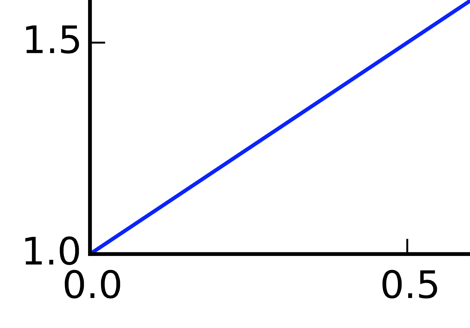
However, I’ve always been frustrated by the quality of the graphics that you get when you export a notebook to PDF. This simple example PDF was exported from a notebook and shows what I mean – and an enlarged screenshot is below:
You can see how blurry the text and lines are – it looks horrible!
Now, normally if I were producing graphs like this in matplotlib, I’d save the outputs as PDF, so I get nice vector graphics which can be enlarged as much as you want without any reduction in quality. However, I didn’t know how I could do that in the notebook while still allowing the plots to be displayed nicely inline while editing the notebook.
Luckily, at the NGCM Summer Academy IPython Training Course, I had the chance to ask one of the core IPython developers about this, and he showed me the method below, which works brilliantly.
All you have to do is add the following code to your notebook – but note, it must be after you have imported matplotlib. So, the top of your notebook would look something like this:
from matplotlib.pyplot import *
%matplotlib inline

from IPython.display import set_matplotlib_formats
set_matplotlib_formats('png', 'pdf')
This tells IPython to store the output of matplotlib figures as both PNG and PDF. If you look at the .ipynb file itself (which is just JSON), you’ll see that it has two ‘blobs’ – one for the PNG and one for the PDF. Then, when the notebook is displayed or converted to a file, the most useful format can be chosen – in this case, the PNG is used for interactive display in the notebook editor, and the PDF is used when converting to LaTeX.
Once we’ve added those lines to the top of our file, the resulting PDF looks far better:
So, a simple solution to a problem that had been annoying me for ages – perfect!
By time this blog post is published, I will have finished my presentation about recipy at EuroSciPy (see the abstract for my talk), and so I thought it would be a good time to introduce recipy to the wider world. I’ve been looking for something like recipy for ages – and I suggested the idea at the Collaborations Workshop 2015 Hack Day. I got together in a team with Raquel Alegre and Janneke van der Zwaan, and our implementation of recipy won the Hack Day prize! I’m very excited about where it could go next, but first I ought to explain what it is:
So, have you ever run a Python script to produce some outputs and then forgotten exactly how you created them? For example, you created plot.png a few weeks ago and now you want to use it in a publication, but you can’t remember how you created it. By adding a single line of code to your script, recipy will log your inputs, outputs and code each time you run the script, and you can then query the resulting database to find out how exactly plot.png was created.
Does this sound good to you? If so, read on to find out how to use it.
Installation is stupidly simple: pip install recipy
Using it is also very simple – just take a Python script like this:
import pandas as pd
from matplotlib.pyplot import *

data = pd.read_csv('data.csv')

data.plot(x='year', y='temperature')
savefig('graph.png')

data.temperature = data.temperature - 273
data.to_csv('output_kelvin.csv')
and add a single extra line of code to the top:
import recipy
import pandas as pd
from matplotlib.pyplot import *
...(code continues as above)...
Now you can just run the script as usual, and you’ll see a little bit of extra output on stdout:
recipy run inserted, with ID 1b40ce05-c587-4f5d-bfae-498e64d71a6c
This just shows that recipy has recorded this particular run of your code.
Once you’ve done this you can query your recipy database using the recipy command-line tool. For example, you can run:
$ recipy search graph.png

Run ID: 1b40ce05-c587-4f5d-bfae-498e64d71a6c
Created by robin on 2015-08-27T20:50:23
Ran /Users/robin/code/euroscipy/recipy/example_script.py using /Users/robin/.virtualenvs/recipypres/bin/python
Git: commit 4efa33fc6e0a81e9c16c522377f07f9bf66384e2, in repo /Users/robin/code/euroscipy, with origin None
Environment: Darwin-14.3.0-x86_64-i386-64bit, python 2.7.9 (default, Feb 10 2015, 03:28:08)
Inputs:
  /Users/robin/code/euroscipy/recipy/data.csv

Outputs:
  /Users/robin/code/euroscipy/recipy/graph.png
  /Users/robin/code/euroscipy/recipy/output_kelvin.csv

** Previous runs creating this output have been found. Run with --all to show. **
You can also view these runs in a GUI by running recipy gui, which will give you a web interface like:
There are more ways to search and find more details about particular runs: see recipy --help for more details. Full documentation is available at Github – which includes information about how this all works under the hood (it’s all to do with the crazy magic of sys.meta_path).
So – please install recipy (pip install recipy), let me know what you think of it (feel free to comment here, or email me at robin AT rtwilson.com), and please submit issues on Github for any bugs you run into (pull requests would be even nicer!).
At the end of the previous post in this series, I was six months into my PhD and worrying that I really needed to come up with an overarching topic/framework/story/something into which all of the various bits of research that I was doing would fit. This part is the story of how I managed to do this, albeit rather slowly!
In fact, I felt that the next year or so of my PhD went very slowly. I can only find a few notes from meetings so I’m not 100% sure what I was spending my time doing, but in general I was trying not to worry too much about the ‘overarching story’ and just get on with doing the research. At this point ‘the research’ was mostly my work on the spatial variability of the atmosphere.
When I first thought about investigating the spatial variability of the atmosphere over southern England I was pretty sure it’d be fairly easy to do: all I had to do was grab some satellite data and do some statistics. I was obviously very naive at that point in my PhD…it was actually far harder than that for a number of reasons. One major problem was that the ‘perfect data’ that I’d imagined didn’t actually exist, and all of the datasets that did exist had limitations. For example, a number of satellite datasets had lots of missing data due to cloud cover, or had poor accuracy, and ground measurements were only taken at a few sparsely distributed points.
I spent a long time writing a very detailed report on the various datasets available, how they were calculated and their accuracy. I then performed independent validations myself (as the accuracy often depended on the situation in which they were used, and I wanted to establish their accuracy over my study area), and finally actually used the datasets to get a rough idea of the spatial variability of these two parameters (AOT and PWC) over southern England. This took a long time, but got me to the stage where I was very familiar with these datasets, and gave me the opportunity to develop my data processing skills.
I then used Py6S – by then a fairly robust tool that was starting to be used by others in the field – to simulate the effects of this spatial variability on satellite images, particularly when atmospheric correction of these images was done by assuming that the atmosphere was spatially uniform. The conclusion of my report was interesting: it basically said that the spatial variability in PWC wasn’t a huge problem for multispectral satellite sensors, but that the spatial variability in AOT could lead to significant errors if it was ignored.
By the time I’d finished writing this report I was probably somewhere between one year and one and a half years into my PhD, and I was wondering where to go next. I’d originally planned that my investigation into the spatial variability of the atmosphere would be one of the ‘three prongs’ of my PhD (yes, I found some notes that I had lost when I wrote the previous article in this series!), and the others would be based around novel sensors (such as LED-based sensors) and BRDF correction of satellite/airborne data. However, I hadn’t really done much on the BRDF side of things, and I wasn’t sure exactly how the LED-based sensors would fit in to my PhD as a lot of the development work was being done by students in the Electronics department, and so I wasn’t sure how much it could be counted as ‘my’ work (I was also concerned that we’d find out that they just didn’t work!).
I spent a lot of time around this point just sitting and thinking, and scribbling vague notes about where I could go next. While doing this I kept coming back to the resolution limitations in methods for estimating AOT from satellite images, for two main reasons.
I really wanted high-resolution data for my investigation into spatial variability, but it wasn’t available so I had to make do with 10km MODIS data instead
My spatial variability work had shown that it was important to take into account the spatial variability in AOT over satellite images, and the only way to do this properly would be to perform a per-pixel atmospheric correction. Of course, a per-pixel atmospheric correction requires an individual estimate for AOT for each pixel in the image: and there weren’t any AOT products that had a high enough resolution to do this for sensors such as Landsat, SPOT or DMC (or up-c0ming sensors such as Sentinel-2).
The obvious answer to this was to develop a way of estimate AOT at high-resolution from satellite data – but I kept well away from this as I was pretty sure it would be impossible (or at least, very difficult, and would require skills that I didn’t have).
I tried to continue with some other work on the novel LED-based instruments, but kept thinking how these instruments would nicely complement a high-resolution AOT product, as they could be used to validate it (after all, if you create a high-resolution product, it is often difficult to find anything to validate it with). Pretty-much everything that I did kept leading me back to the desire to develop a high-resolution AOT product…
I eventually gave up trying to resist this, and started brainstorming possible ways to approach creating a high-resolution AOT product. I was pretty sure that none of the ‘standard’ approaches would work (people had tried these before and hadn’t succeeded) so I tried to think ‘outside the box’. I eventually came up with an idea – and you’ll have to wait for the next part to find out what this idea was, how I ‘sold’ it to my supervisors, and what happened next.
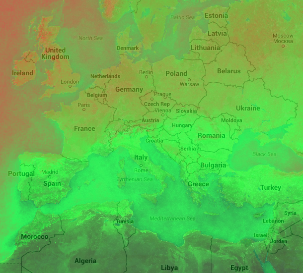
Summary: I’ve developed an interactive cloud frequency map, available here. It may be particularly useful for satellite imaging researchers working out where they can acquire imagery easily.
One of the major issues with optical satellite imaging is that you can’t see through clouds: so normally when its cloudy, you can’t get anything useful from your images. This actually has a big effect on where you can use satellite imaging effectively: for example, a lot of people have used satellite data to monitor changes in the Amazon rainforest, but it’s quite challenging to find cloud-free images due to the climate in that region of the world.
Similarly, I remember a friend of mine struggling throughout his PhD with cloud cover. He was trying to observe vegetation in India, and needed to look at images taken around the monsoon because the vegetation was growing most vigorously at that time of year. The problem, of course, is that its very cloudy during the monsoon season – so there were barely any images he could use, and he ended up spending half of his PhD developing a new method to classify cloud from his images, so that he could extract the small fraction of the data that was actually usable. I’ve run into similar problems too – for example, some research in Hydrabad ran into problems caused by the limited availability of data due to cloud cover.
I’ve often found myself wanting to look at cloud frequency in different areas so that when I have a number of options for where to use as a case study for something, I can easily pick the area that is likely to have the most cloud-free data available. I’ve been a ‘Trusted Tester’ of Google Earth Engine for a long time, and had written a short script in Earth Engine to produce a map of cloud frequency.
I found myself using this frequently with colleagues, but I wasn’t able to share the data or interface with anyone easily. So, a few weekends ago I sat down and altered one of the EarthEngine demonstration applications (the ‘trendy-lights’ demo) to work with my cloud frequency code. After a bit of trial and error I got it working: the webapp is available here, and the code is on Github. I’m fairly new to Javascript development, but I think it all works fairly well: you should be able to search to find a location on the map, and you can click anywhere on the map to produce a pop-up box with the cloud cover percentage. The higher this percentage, the more days in a year are considered to be cloudy by the MODIS satellite (more details are available from the Info link in the top right).
So, I hope you find this useful (and even if you’re not using it as a satellite imaging researcher, you may find the cloud cover patterns across the world to be fascinating anyway…)