I just shared this approach with some friends, and thought I’d blog it here too.
When I get a relatively small amount of monetary compensation for something, I take the ‘Feynman Approach’ to it and buy something fun with the money, giving me a sense of satisfaction from the compensation (which, presumably, was to compensate me for something bad that happened).
Now, it’s some dopey legal thing, but when you give the patent to the government, the document you sign is not a legal document unless there’s some exchange, so the paper I signed said,
"For the sum of one dollar, I, Richard P. Feynman, give this idea to the government . . ."
I sign the paper.
"Where’s my dollar?"
…[he eventually gets the dollar]
I take the dollar, and I realize what I’m going to do. I go down to the grocery store, and I buy a dollar’s worth – which was pretty good, then – of cookies and goodies, those chocolate goodies with marshmallow inside, a whole lot of stuff.
I come back to the theoretical laboratory, and I give them out: "I got a prize, everybody! Have a cookie! I got a prize! A dollar for my patent! I got a dollar for my patent!"
…[everyone else wants to get a real dollar for their patent]
I don’t usually spend the compensation amount on sweets or baked goods (unless it’s really quite small), but I often buy myself a little something I wanted for fun – like a few electrical components, a 3D printing accessory (or filament), or just a second-hand book (or a new one if the amount is enough).
Recent bits of compensation I’ve used this approach with are mostly Delay Repay for delayed trains (it means I was inconvenienced by the train delay, so I ‘deserve’ something nice), but it can apply to other things too. I don’t usually apply it if the compensation is reasonably large, and obviously not if I’m really short of money (in that case the money goes into ‘general funds’), but for compensation less than £15-20 it’s often an approach I take.
(I should point out that I definitely don’t agree with Feynman on everything, particularly some of his views on women, but in general I enjoyed his books)
Summary: I’m involved in organising a hackathon, and I’d love you to take part. The open-source GeoTAM hackathon focuses on estimating turnover for individual business locations in the UK, from a variety of open datasets. Please checkout the hackathon page and sign up. There are prizes of up to £2,000!
(Click image for a larger version)
I’m currently working with Rebalance Earth, a boutique asset manager who are focused on making nature an investable asset. Our aim is to mobilise investment in UK natural infrastructure – for example, by arranging investment to undertake river restoration and reduce the risk of flooding. We will do this by finding businesses at risk of flooding, designing restoration schemes that will reduce this risk, and setting up ‘Nature-as-a-Service’ contracts with businesses to pay for the restoration.
I’m the Lead Geospatial Developer at Rebalance Earth, and am leading the development of our Geospatial Predictive Analytics Platform (GPAP), which helps us assess businesses at risk of flooding and design schemes to reduce this flooding.
An important part of deciding which areas to focus on is estimating the total business value at risk from flooding. A good way of establishing this is to use an estimate of the business turnover. However, there are no openly-available datasets showing business turnover in the UK – which is where the hackathon comes in.
We’re looking for participants to bring their expertise in programming, data science, machine learning and more to take some datasets we provide, combine them with other open data and try and estimate turnover. Specifically, we’re interested in turnover of individual business locations – for example, the turnover of a specific supermarket, not the whole supermarket chain.
The hackathon runs from 20th – 26th November 2024. We’ll provide some datasets, some ideas, and a Discord server to communicate through. We’d like you to bring your expertise and see what you can produce. This is a tricky task, and we’re not expecting fully polished solutions; proof-of-concept solutions are absolutely fine. You can enter as a team or an individual.
Most importantly, there are prizes:
£2,000 for the First Prize
£1,000 for the Second Prize
£500 for the Third Prize
and there’s a possibility that we might even hire you to continue work on your idea!
A quick post today to talk about a couple of PostGIS functions I learnt recently.
I had a CSV file that contained well-known binary (WKB) representations of geometries, stored as hexadecimal strings. I imported the CSV into a PostGIS database, and wanted to convert these to be proper PostGIS geometries.
I initially went for the ST_GeomFromWKB function, but kept getting an error that the function didn’t exist. Well, actually the error said that it couldn’t find a function that exists with that name and those specific parameter types. That’s because I was calling it with the text column containing the hex strings, and the documentation for ST_GeomFromWKB says that its signature is one of:
So, we need to convert the hexadecimal string to a bytea type – that is, a proper set of bytes. We can do this using the decode function, which takes two parameters: the text to decode, and a format specifier which must be one of base64, escape or hex. In this case, we’re decoding a hex string, so we want the latter.
Putting this together, we can write some simple SQL that does what we want. First, we create a geom column in our table:
ALTER TABLE test ADD geom Geometry;
and then we set that column to be the result of decoding the hex and converting the WKB to a geometry:
UPDATE test SET geom = ST_GeomFromWKB(decode(wkb_column, 'hex'), 4326);
Note that here I knew that my WKB was encoding a point in the WGS84 latitude/longitude co-ordinate system, so I passed the EPSG code 4326 which refers to this co-ordinate system.
It’s been a while since I posted here – I kind of lost momentum over the summer (which is a busy time with a school-aged child) and never really picked it up again.
Anyway, I wanted to write a quick post to tell people that I won two awards at the British Cartographic Society awards ceremony a few weeks ago.
They were both for my British Placename Mapper web app, which is described in more detail in this blog post. If you haven’t seen it already, I strongly recommend you check it out.
I won a Highly Commended certificate in the Avenza Award for Electronic Mapping, and the First Prize trophy for the Ordnance Survey Award (for any map using OS data).
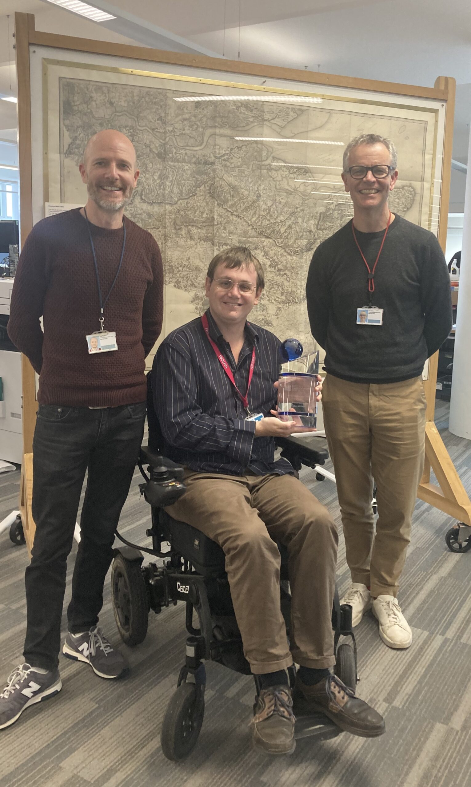
The certificates came in a lovely frame, and the trophy is enormous – about 30cm high and weighing over 3kg!
Here’s the trophy:
I was presented with the trophy at the BCS Annual Conference in London, but they very kindly offered to keep the trophy to save me carrying it across London on my wheelchair and back on the train, so they invited me to Ordnance Survey last week to be presented with it again. I had a lovely time at OS – including 30 minutes with their Director General/CEO and was formally presented with my trophy again (standing in front of the first ever Ordnance Survey map!):
Full information on the BCS awards are available on their website and I strongly recommend submitting any appropriate maps you’ve made for next year’s awards. I need to get my thinking cap on for next year’s entry…
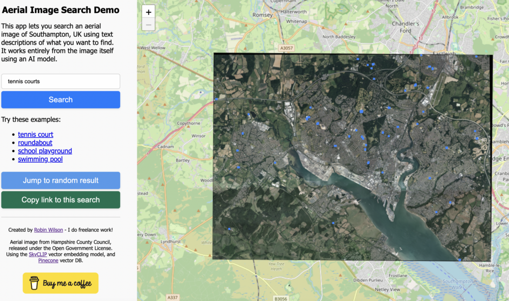
Summary: I’ve created a demo web app where you can search an aerial photo of Southampton, UK using text queries such as "roundabout", "tennis court" or "ship". It uses vector embeddings to do this – which I explain in this blog post.
In this post I’m going to try and explain a bit more about how this works.
Firstly, I should explain that the only data used for the searching is the aerial image data itself – even though a number of these things will be shown on the OpenStreetMap map, none of that data is used, so you can also search for things that wouldn’t be shown on a map (like a blue bus)
The main technique that lets us do this is vector embeddings. I strongly suggest you read Simon Willison’s great article/talk on embeddings but I’ll try and explain here too. An embedding model lets you turn a piece of data (for example, some text, or an image) into a constant-length vector – basically just a sequence of numbers. This vector would look something like [0.283, -0.825, -0.481, 0.153, ...] and would be the same length (often hundreds or even thousands of elements long) regardless how long the data you fed into it was.
In this case, I’m using the SkyCLIP model which produces vectors that are 768 elements long. One of the key features of these vectors are that the model is trained to produce similar vectors for things that are similar in some way. For example, a text embedding model may produce a similar vector for the words "King" and "Queen", or "iPad" and "tablet". The ‘closer’ a vector is to another vector, the more similar the data that produced it.
The SkyCLIP model was trained on image-text pairs – so a load of images that had associated text describing what was in the image. SkyCLIP’s training data "contains 5.2 million remote sensing image-text pairs in total, covering more than 29K distinct semantic tags" – and these semantic tags and the text descriptions of them were generated from OpenStreetMap data.
Once we’ve got the vectors, how do we work out how close vectors are? Well, we can treat the vectors as encoding a point in 768-dimensional space. That’s a bit difficult to visualise – so imagine a point in 2- or 3-dimensional space as that’s easier, plotted on a graph. Vectors for similar things will be located physically closer on the graph – and one way of calculating similarity between two vectors is just to measure the multi-dimensional distance on a graph. In this situation we’re actually using cosine similarity, which gives a number between -1 and +1 representing the similarity of two vectors.
So, we now have a way to calculate an embedding vector for any piece of data. The next step we take is to split the aerial image into lots of little chunks – we call them ‘image chips’ – and calculate the embedding of each of those chunks, and then compare them to the embedding calculated from the text query.
I used the RasterVision library for this, and I’ll show you a bit of the code. First, we generate a sliding window dataset, which will allow us to then iterate over image chips. We define the size of the image chip to be 200×200 pixels, with a ‘stride’ of 100 pixels which means each image chip will overlap the ones on each side by 100 pixels. We then configure it to resize the output to 224×224 pixels, which is the size that the SkyCLIP model expects as input.
We then iterate over all of the image chips, run the model to calculate the embedding and stick it into a big array:
dl = DataLoader(ds, batch_size=24)

EMBEDDING_DIM_SIZE = 768
embs = torch.zeros(len(ds), EMBEDDING_DIM_SIZE)

with torch.inference_mode(), tqdm(dl, desc='Creating chip embeddings') as bar:
    i = 0
    for x, _ in bar:
        x = x.to(DEVICE)
        emb = model.encode_image(x)
        embs[i:i + len(x)] = emb.cpu()
        i += len(x)

# normalize the embeddings
embs /= embs.norm(dim=-1, keepdim=True)

embs.shape
We also do a fair amount of fiddling around to get the locations of each chip and store those too.
Once we’ve stored all of those (I’ll get on to storage in a moment), we need to calculate the embedding of the text query too – which can be done with code like this:
text = tokenizer(text_queries)
with torch.inference_mode():
        text_features = model.encode_text(text.to(DEVICE))
        text_features /= text_features.norm(dim=-1, keepdim=True)
        text_features = text_features.cpu()
It’s then ‘just’ a matter of comparing the text query embedding to the embeddings of all of the image chips, and finding the ones that are closest to each other.
To do this, we can use a vector database. There are loads of different vector databases to choose from, but I’d recently been to a tutorial at PyData Southampton (I’m one of the co-organisers, and I strongly recommend attending if you’re in the area) which used the Pinecone serverless vector database, and they have a fairly generous free tier, so I thought I’d try that.
Pinecone, like all other vector databases, allows you to insert a load of vectors and their metadata (in this case, their location in the image) into the database, and then search the database to find the vectors closest to a ‘search vector’ you provide.
I won’t bother showing you all the code for this side of things: it’s fairly standard code for calling Pinecone APIs, mostly copied from their tutorials.
I then wrapped this all up in a FastAPI API, and put a simple Javascript front-end on it to display the results on a Leaflet web map. I also added some basic caching to stop us hitting the Pinecone API too frequently (as there is limit to the number of API calls you can make on the free plan). And that’s pretty-much it.
I hope the explanation made sense: have a play with the app here and post a comment with any questions.
I’m interested to find out who is reading my blog. Following the lead of Jamie Tanna who was in turn copying Terence Eden (both of whose blogs I read), I’d like to ask people who read this to drop me an email or leave a comment on this post if you read this blog and see this post. I have basic analytics on this blog, and I seem to get a reasonable number of views – but I don’t know how many of those are real people, and how many are bots etc.
Feel free to just say hi, but if you have chance then I’d love to find out a bit more about you and how you read this. Specifically, feel free to answer any or all of the following questions:
Do you read this on the website or via RSS?
Do you check regularly/occasionally for new posts, or do you follow me on social media (if so, which one?) to see new posts?
How did you find my blog in the first place?
Are you interested in and/or working in one of my specialisms – like geospatial data, general data science/data processing, Python or similar?
Which posts do you find most interesting? Programming posts on how to do things? Geographic analyses? Book reviews? Rare unusual posts (disability, recipes etc)?
Have you met me in real life?
Is there anything particular you’d like me to write about?
The comments box should be just below here, and my email is robin@rtwilson.com
For months now I’ve been collecting a load of links saying that I’ll get round to blogging them "soon". Well, I’m currently babysitting for a friend’s daughter (who is sleeping peacefully upstairs), so I’ve finally found time to write them up.
So, here are a load of links – a lot of them are geospatial- or data-related, but I hope you might find something here you like even if those aren’t your specialisms:
QGIS Visual Changelog for v3.36 – QGIS is great GIS software that I use a lot in my work. The reason this link is here though is because of their ‘visual changelog’ that they write for every new version – it is a really good way of showing what has changed in a GUI application, and does a great job of advertising the new features.
List of unusual units of measurement – a fascinating list from Wikipedia. I think my favourite are the barn (and outhouse/shed) and the shake – you’ll have to read the article to see what these are!
List of humourous units of measurement – linked from the above is this list of humourous units of measurement, including the ‘beard-second’, and the Smoot.
lonboard – a relatively new package for very efficiently creating interactive webmaps of geospatial data from Python. It is so much faster than geopandas.explore(), and is developing at a rapid pace. I’m using it a lot these days.
A new metric for measuring learning – an interesting post from Greg Wilson about the time it takes learners to realise that something was worth learning. I wonder what the values are for some things that I do a lot of – remote sensing, GIS, Python, cloud computing, cloud-native geospatial etc.
CyberChef – from GCHQ (yes, the UK signals intelligence agency) comes this very useful web-based tool for converting data formats, extracting data, doing basic image processing, extracting files and more. You can even build multiple tools into a ‘recipe’ or pipeline.
envreport – a simple Python script to report lots of information about the Python environment in a diffable form – I can see this being very useful
Antarctic glaciers named after satellites – seven Antarctic glaciers have been named after satellites, reflecting (ha!) the importance of satellites in monitoring Antarctica
MoMAColors and MetBrewer – these are color palettes derived from artwork at the Museum of Modern Art and the Metropolitan Museum of Art in New York. There are some beautiful sets of colours in here (see below) which I want to use in some future data visualisations.
geospatial-cli – a list of geospatial command-line tools. Lots of them I knew, but there were some gems I hadn’t come across before here too.
map-gl-tools – a nice Javascript package to add a load of syntactic sugar to the MapLibreJS library. I’ve recently started using this library and found things quite clunky (coming from a Leaflet background) so this really helped
CoolWalks – a nice research paper looking at creating walking routes on the shaded side of the street for various cities
Writing efficient code for GeoPandas and Shapely in 2023 – a very useful notebook showing how to do things efficiently in GeoPandas in 2023. There are a load of old ways of doing things which are no longer the most efficient!
Towards Flexible Data Schemas – this article shows how the flexibility of data schemes in specifications like STAC really help their adoption and use for diverse purposes
I’ve been informed that this method is no longer working, and I haven’t had time to try and update it to work again. I’m leaving this here for historical value, and in case anyone can adapt the method to make it work.
Microsoft Planetary Computer is a wonderful archive of geospatial datasets (primarily raster images of various types), provided with a STAC catalog to enable them to be easily searched through an API. That’s fine for normal usage where you want to find a selection of images and access the images themselves, but less useful when you want to do some analysis of the metadata itself.
For that use case, Planetary Computer provide the STAC metadata in bulk, stored as GeoParquet files. Their documentation page explains how to use this with geopandas and do some large-ish scale processing with Dask. I wanted to try this with DuckDB – a newer tool that is excellent at accessing and processing Parquet files, including efficiently accessing files available via HTTP, and only downloading the relevant parts of the file. So, this post explains how I managed to do this – showing various different approaches I tried and how (or if!) each of them worked.
Getting URLs
Planetary Computer URLs are basically just URLs to files on Azure Blob Storage. However, the URLs require signing with a Shared Access Signature (SAS) key. Luckily, there is a Planetary Computer Python module that will use an API to generate the correct keys for us.
In the docs for using the STAC GeoParquet files, they give this code:
This gets a collection, and the geoparquet-items collection-level asset, having used a ‘modifier’ to sign the URLs as they are acquired from the STAC API. The URL is then stored in asset.href.
Using the DuckDB CLI – with HTTP URLs
When using GeoPandas, the docs show that you can pass a storage_options parameter to the read_parquet method and it will ‘just work’:
However, to use the file in DuckDB we need a full URL. The SQL code we’re going to use in DuckDB for a quick test looks like this:
SELECT * FROM <URL> LIMIT 1
This just gets the first row of whatever URL is given.
Unfortunately, though, the URL provided by the STAC catalog looks like this:
abfs://items/io-lulc-9-class.parquet
If we try that with DuckDB, we find it doesn’t know how to deal with it. So, we need to convert this to a standard HTTP URL that can be downloaded as if it were just typed into a web browser (or used with cURL or wget). After a bit of playing around, I found I could create a full URL with this Python code:
That’s taking the account_name and sticking it in as part of the host part of the UK, then extracting the path from the original URL and adding that, and then finishing with the SAS token (stored as credential in the storage options) as a URL query parameter.
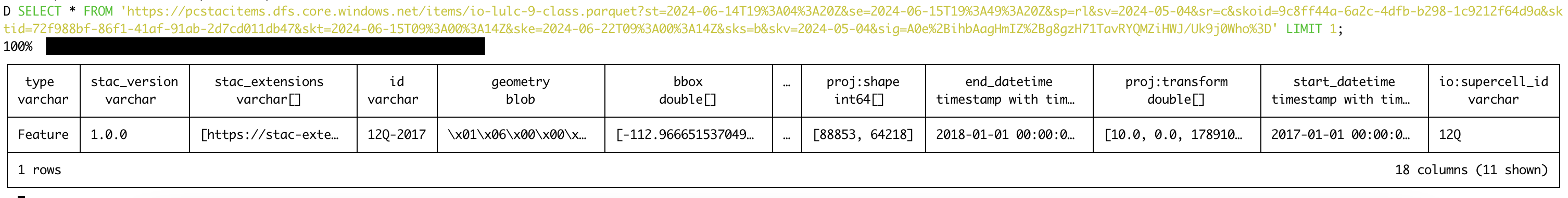
That results in a URL that looks like this (split over multiple lines for readability):
(note: that specific URL won’t work for you, as the SAS tokens are time-limited).
If we insert that into our DuckDB SQL statement then we find it works (click to enlarge):
Great! Now let’s try with a different collection on Planetary Computer – in this case the Sentinel 2 collection. We can make the URL in the same way as before, by changing how we define asset:
and then using the same query in DuckDB with the new URL. Unfortunately, this time we get an error:
Invalid Input Error: File '<URL>' too small to be a Parquet file
The problem here is that for larger collections, the STAC metadata is spread out over a series of GeoParquet files inside a folder, and the URL we’ve been given is just to the folder (even though it ends in .parquet). As we’re just using HTTP, there is no way to do things like list the files in a folder, so DuckDB has no way to find out what files are within the folder and start reading them. We need to find another way.
Using the DuckDB CLI – with the Azure extension
Conveniently, there is an Azure extension for DuckDB, and it lets you use URLs like 'abfss://⟨my_filesystem⟩/⟨path⟩/⟨my_file⟩.⟨parquet_or_csv⟩'. That’s a slightly different URL scheme to the one we’ve been given (abfss as opposed to abfs), but we can easily sort that.
Looking at the authentication docs though, it seems to require you to specify either a connection string, a service principal or using the ‘Azure Credential Chain’ (which, I think, works with the az command line and various environment variables that you may have set up). We don’t have any of those – they’re all a far broader scope than what we’ve got, which is just a SAS token for a specific file or folder. It looks like the Azure extension doesn’t support this, so we’ll have to look for another way.
Using the DuckDB Python library – with an Azure connector
As well as the command-line interface, DuckDB can also be used from Python. To set this up, just run pip install duckdb. While you’re at it, you might want to install pandas and the adlfs library for connecting to Azure Storage.
Using this is actually quite simple, first import the libraries:
import duckdb
from adlfs.spec import AzureBlobFileSystem
then set up the Azure connection:
a = AzureBlobFileSystem(account_name='pcstacitems',
   sas_token=asset.extra_fields["table:storage_options"]['credential'])
Note how here we’re using the sas_token parameter to provide a SAS token. We could use a different parameter here to provide a connection string or some other credential type. I couldn’t find much real-world use of this sas_token parameter when looking online – so this is probably the key ‘less well documented’ bit to take away from this article.
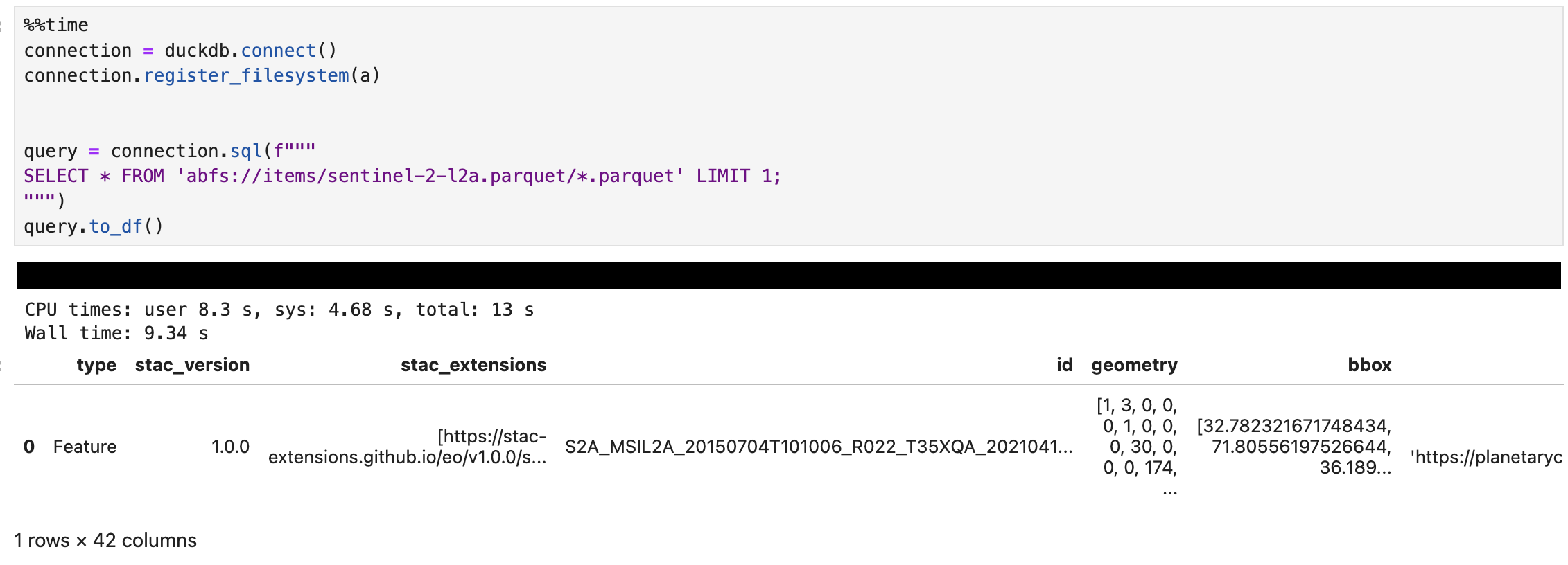
Continuing, we then connect to DuckDB and ‘register’ this Azure connection:
The call to to_df at the end converts the result into a Pandas DataFrame for easy viewing and manipulation. The results are shown below (click to enlarge):
Note that we’re passing a URL of abfs://items/sentinel-2-l2a.parquet/*.parquet – this is the URL from the STAC catalog with /*.parquet added to the end to ensure DuckDB picks up the large number of Parquet files stored there. I’d have thought this would have worked without that, but if I miss that out I get a error saying:
TypeError: int() argument must be a string, a bytes-like object or a real number, not 'NoneType'
I suspect this is something to do with how things are passed to the Azure connection that we registered with DuckDB, but I’m not entirely sure. If you do know, then please leave a comment!
A few fun queries
So, now we’ve got this working, what can we do? Well, we can – fairly efficiently – run queries across all the STAC metadata for Sentinel 2 images. I’ll just give a few examples of queries I’ve run below.
We can find out how many images there are in the collection in total:
SELECT COUNT(*) FROM 'abfs://items/sentinel-2-l2a.parquet/*.parquet'
We can do the same for just the images acquired in 2020 – by using a fact we know about how the individual parquet files are named (from the Planetary Computer docs):
SELECT COUNT(*) FROM 'abfs://items/sentinel-2-l2a.parquet/*2020*.parquet'
And we can start looking at how many scenes were captured with different amounts of cloud cover:
SELECT COUNT(*) / (SELECT COUNT(*) FROM 'abfs://items/sentinel-2-l2a.parquet/*2020*.parquet'), CASE
    WHEN "eo:cloud_cover" between 0 and 5 then '0-5%'
    WHEN "eo:cloud_cover" between 5 and 10 then '5-10%'
    WHEN "eo:cloud_cover" between 10 and 15 then '10-15%'
    END AS category
FROM 'abfs://items/sentinel-2-l2a.parquet/*2020*.parquet' GROUP BY category,
This tells us that 20% of scenes had between 0 and 5% cloud cover (quite a high number, I thought – but then again, I am used to living in the UK!), and around 4-5% in each of the 5-10% and 10-15% categories.
There are plenty of other analyses that you could do with these Parquet files, of course. At some point I might even get around to the task which initially made me look into this: that is, trying to find Landsat and Sentinel 2 scenes that were acquired over the same location at very similar times. I think I’ll leave that for another day though…
Another new-ish package that I’ve never got around to writing about on my blog is offline_folium. It has a somewhat niche use-case, but it seems like a few people have found it useful.
In brief, it allows you to use the folium package for creating interactive maps from Python, but without an internet connection. Folium is built on top of the Leaflet web mapping library – and it loads all the relevant JS and CSS files directly from CDNs. This means that if you try and use folium without an internet connection it just doesn’t work. Offline_folium works around this by downloading the files when you do have an internet connection, and then re-writing the links to the files to point to the offline versions.
I originally created this package when doing freelance work on a project for the UK Navy – they wanted to have interactive maps on an air-gapped computer, so I built a system that would allow this (in this case, the JS/CSS file download step was run as part of building the ‘app’ we produced). I should note at this point that without an internet connection the default OpenStreetMap background mapping will not work. In some situations that would be a significant problem – but we were using other background mapping, coastline vector files and so on, so it wasn’t a problem for us.
So, how do you use this package?
First, install it using pip install offline_folium. Then make sure you have an internet connection and run python -m offline_folium – this will download the JS/CSS files and store them in a sensible place (chosen automatically). Now you’re all set up.
Once you have no internet connection and want to use folium, you must import it in a slightly different way – first import offline from offline_folium, and then import folium, like this:
from offline_folium import offline
import folium
Now you can use folium as usual, for example by creating a simple map object:
m = folium.Map()
So, that’s pretty-much it. People are actively submitting pull requests at the moment, so hopefully the functionality will expand to work with various folium plugins too.
For more information (or to submit a PR yourself), see the Github repo.
I realised recently that I’d never actually blogged about my pyAURN package – so it’s about time that I did.
When doing some freelance work on air quality a while back, I wanted an easy way to access UK air quality from the Automatic Urban and Rural Network (AURN). Unfortunately, there isn’t a nice API for accessing the data. Strangely, though, they do provide the data in a series of RData files for use by the openair R package. I wanted to use the data from Python though – but conveniently there is a Python package for reading RData files.
So, I put all these together into a simple Python package called pyAURN. It is strongly based upon openair, but is a lot more limited in functionality – it basically only covers importing the data, and doesn’t have many plotting or analysis functions.
Here’s an example of how to use it:
from pyaurn import importAURN, importMeta, timeAverage

# Download metadata of site IDs, names, locations etc
metadata = importMeta()

# Download 4 years of data for the Marylebone Road site
# (MY1 is the site ID for this site)
# Note: range(2016, 2022) will produce a list of six years: 2016, 2017, 2018, 2019, 2020, and 2021.
# Alternatively define a list of years to use eg. [2016,2017,2018,2019,2020,2021]
data = importAURN("MY1", range(2016, 2022))

# Group the DataFrame by a frequency of monthly, and the statistic mean().
data_monthly = timeAverage(data,avg_time="month",statistic="mean")
I found this really useful for my air quality analysis work – and I hope you do too. The package is on PyPI, so you can run pip install pyaurn or view the project on Github.