Robin's Blog

Roadside leafiness from space – Part 1

If you just want to see some pretty maps of roadside leafiness then scroll down…otherwise, start at the top to find out how I did this.

I’ve recently started doing a little bit of satellite imaging work again, and started off with a project that was inspired by a post on James O’Connor’s blog. He posted about looking at the leafiness of streets in cities by extracting the NDVI (Normalized Difference Vegetation Index) within 20m of a road. He did this for Cleveland, Ohio using data from the Landsat 5 sensor, and produced a nice output map showing some interesting patterns.

This caught my interest, and I decided to see if I could scale up the analysis to larger areas. My go-to tool for doing simple but large-scale remote sensing work is Google Earth Engine – a free tool provided by Google which can easily process large volumes of satellite imagery stored on Google’s servers. To use this tool you have to be a ‘registered tester’, as the tool is not fully released yet, but it is easy to register to become a tester.

For this particular task I needed two datasets: some relatively high-resolution satellite imagery to use to calculate the NDVI, and some vector data of the road network. Conveniently, Google Earth Engine already contains datasets that fulfil these criteria: all of the Sentinel-2 data is in there, which provides visible and near-infrared bands at 10-30m resolution (depending on the band – the ones that we need for NDVI calculation are provided at 10m), and the TIGER Roads dataset containing vector data on roads across the USA. I thought this would give me a good starting point – although I was keen to perform this analysis for the UK, so I decided to find an equivalent vector roads dataset for the UK. I downloaded OS Open Roads, and then uploaded it to Earth Engine so it could be used in my analysis. (Actually, there was a bit more to it than this, as the Open Roads data is provided in 100km tiles, so I had to stitch all of these together before uploading – I really wish OS would provide the data in a single large file. I then ran into various problems with projections – see my questions to the Google Earth Engine developers – but eventually managed to get a reasonable accuracy by uploading in the WGS-84 projection.)

The code to perform the analysis is actually very simple, and is shown below. For those of you who have access to Earth Engine, this link will open the code up in the Earth Engine workspace. In summary, what we do is select all of the Sentinel-2 data for 2017, and take the pixel-wise median (this is a very crude way of filtering out clouds, shadows and other anomalies – leaving a relatively representative view of the ground). We then calculate the NDVI and extract pixels within 10m of a road (I chose 10m as this was more likely to just get vegetation that was at the edge of the road, and was possible as Sentinel-2 is a higher resolution sensor than Landsat 5). The easiest way to do this extraction is to create a raster of distance from the vector roads data (putting in a small maximum distance to search to increase computational efficiency) and then use this to mask the NDVI. Finally, we visualise the data on the map provided in the Earth Engine workspace, and download it as a GeoTIFF for further analysis.

var roads = ee.FeatureCollection("TIGER/2016/Roads"),
    sentinel2 = ee.ImageCollection("COPERNICUS/S2"),
    roads_uk = ee.FeatureCollection("users/rtwilson/RoadLink_All_WGS84"),

var roads_uk_fc = ee.FeatureCollection(roads_uk);

// Load Sentinel collection, filter to 2017, select B4 (Red) and B8 (NIR)
// and create a median composite
var s2_median = sentinel2
                .filterDate('2017-01-01', '2017-12-31')
                .select(['B4', 'B8'])
                .median();

// Calculate NDVI
var ndvi = s2_median.normalizedDifference(['B8', 'B4']).rename('NDVI');

// Calculate distance from road for each pixel
// The first parameter (10) is the maximum distance to look, in metres
// Looking 10m in each direction gives a buffer of 20m
var dist = roads_uk_fc.distance(10)

// Threshold the distance to a road to get a binary image for masking with
var thresh_distance = dist.lt(10);

// Use the distance threshold image to mask the NDVI
// var masked_ndvi = ndvi.mask(thresh_distance);
var masked_ndvi = ndvi.multiply(thresh_distance);

Map.addLayer(masked_ndvi, {}, 'NDVI near roads');

// Export the image, specifying scale and region.
Export.image.toDrive({
  image: masked_ndvi,
  description: 'Masked_NDVI',
  scale: 10,
  region: area_to_export,
  crs: "EPSG:27700",
  maxPixels: 8185883500
});

This further analysis was carried out in QGIS – and there are a few more posts coming on some issues that I ran into while doing the QGIS-analysis, and a few tips of useful GDAL functionality that can help with this sort of analysis. In this post I’m going to focus on the visualisation I did and show some pretty pictures. In the next post I will show a bit more quantitative analysis comparing leafiness across settlements in the UK.

Anyway, on to the pictures. I used the viridis colourmap as this is generally a well-designed colourmap, and quite appropriate in this context as the high values are green/yellow. The first set of images below are all on the same colour scale, so you can compare colours across the images.

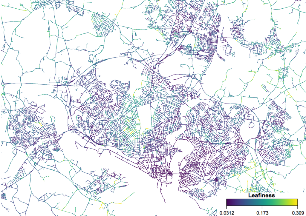
First, of course, I looked at my home town, Southampton:

You can see some interesting patterns here. There is a major area of high leafiness in the Upper Shirley area, to the west of the common, with some high areas also in Highfield and Bassett. Most of the city centre was very low – interestingly, even including the areas around the major parks – and most of the other areas of the city were quite low as well. There seems to be a relationship between leafiness and the wealth of an area, with relatively wealthy areas having high leafiness and relatively poor areas having low leafiness – as you’d expect.

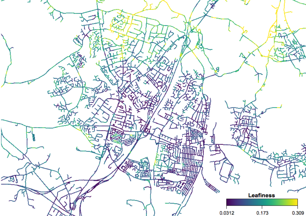
Moving slightly north to Eastleigh and Chandlers Ford, you see a very noticeable hot spot:

The area of Hiltingbury, at the northern end of Chandlers Ford, is very leafy – which definitely matches up with my experience visiting there! In general, the western side of Chandlers Ford is leafier, with the eastern side of Chandlers Ford having almost as low values as Eastleigh. In general Chandlers Ford is considered significantly more desirable than Eastleigh, so I’m slightly surprised that there isn’t more of a difference. The centre of Eastleigh is extremely low – as these streets are mostly terraced or semi-detached houses with little vegetation around (either trees or front gardens) – but again, I’m slightly surprised to see the hot spot on the west of Eastleigh.

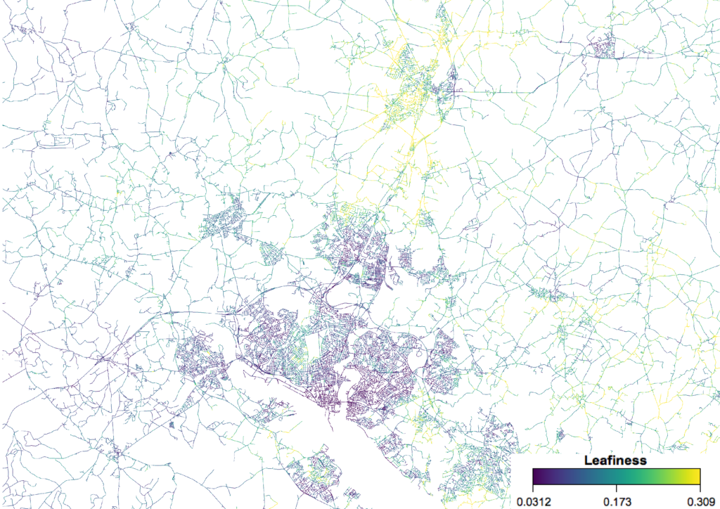
Zooming out to encompass multiple settlements in southern Hampshire, we see a very obvious pattern:

Winchester is completely dominating the area, with far higher values even than most rural areas. Again, this matches up with expectations given that Winchester is a wealthy city, and is known as a nice, leafy place to live. The rural area between Eastleigh and Winchester is also very high, as is – slightly surprisingly – the area around Bursledon to the east of Southampton.

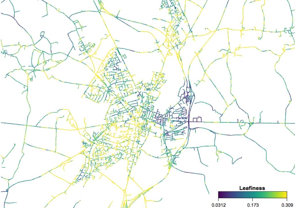
Zooming in on Winchester shows the pattern within the city:

There is a significant east-west divide, with the estates of detached houses that have grown up on the west of the city having very high leafiness, and the older terraced and semi-detached areas on the east of the city having a far lower leafiness.

So, there are some interesting patterns here and some pretty maps. In Part 2, I’ll look at some statistical analysis of leafiness across the England, Wales and Scotland, and then consider some of the limitations of this approach.

If you found this post useful, please consider buying me a coffee.
This post originally appeared on Robin's Blog.

Tagged with:

Categorised as: Academic, GIS, Programming, Remote Sensing