I recently saw Michael Galloy’s post at http://michaelgalloy.com/2016/02/18/ten-little-idl-programs.html, showing some short (less than ten lines long) programs in IDL. I used to do a lot of programming in IDL, but have switched almost all of my work to Python now – and was intrigued to see what the code looked like in Python.
I can’t guarantee that all of my Python code here will give exactly the same answer as the IDL code – but the code should accomplish the same aim. I’ve included the IDL code that Michael provided, and for each example I provide a few comments about the differences between the Python and IDL code. I haven’t shown the output of the IDL examples in the notebook (yes, I know I can run IDL through the Jupyter Notebook, but I don’t have that set up on this machine.
Firstly, we import the various modules that we need for Python. This is rather different to IDL, where all of the functionality for these programs is built in – but is not necessarily a disadvantage, as it allows an easier separation of functionality, allowing you to only include the functions you need. I’m going to ‘cheat’ slightly, and not count these import lines in the number of lines of code used below – which I think is fair.
It is also worth noting that counting the number of lines of a bit of Python code is rather arbitrary – because although whitespace is syntactically important, you can still often combine multiple lines into one line. For example:
a=5;b=10;print(a+b)
15
Here I’m going to keep to writing Python in a sensible, relatively standard (hopefully PEP8 compliant) way.
1 line: output, calling a procedure:
IDL
print,'Hello, world!'
Python
print("Hello, world!")
Hello, world!
These are almost exactly the same…not much to see here!
2 lines: assignment, calling a function, system variables, array operations, keywords:
This is fairly similar, the major differences being the use of the np. prefix on various functions as they are part of the numpy library (this can be avoided by importing numpy as from numpy import *, but that is not recommended). The only other real differences are the use of a function to convert from degrees to radians, rather than a constant conversion factor, and the differences in the name of the function that produces an array containing a range of values – I personally found findgen always made me thinking of FINDing something, rather than Floating INDex GENeration, but that’s just me!
3 lines: input, output format codes:
IDL
name=''read,'What is your name? ',nameprint,name,format='("Hello, ", A, "!")'
Python
name=input('What is your name? ')print("Hello {name}!".format(name=name))
What is your name? Robin
Hello Robin!
This is the first example where the lengths differ – and Python is very slightly shorter. The only reason for this is that IDL requires you to initialise the name variable before you can read into it, whereas Python does not. I prefer the way that the formatting of the string works in Python – although this is but one of multiple ways of doing it in Python. For reference, you could also do any of the following:
This example is also slightly shorter in Python, mainly because we don’t have to create the display window manually, and therefore we don’t need to find out the size of the image before-hand. On the other hand, Python has no way to set the title of a plot in the call to the plotting function (in this case imshow, which I personally think is a more understandable name than tv), which adds an extra line.
6 lines: logical unit numbers, read binary data, contour plots, line continuation:
<matplotlib.contour.QuadContourSet at 0x1182a4c50>
This is also shorter, although I must admit that I haven’t configured the contour levels manually as was done in the IDL code – as I often find I don’t need to that. Again, you can see that we don’t need to create the array before we read in the file, and we don’t have to deal with all of the opening, reading and closing of the file as the np.fromfile function does all of that for us. (If we did want to work at a lower level then we could – using functions like open and close). I’ve also shown a line continuation in Python, which in many circumstances works with no explicit ‘continuation characters’ – even though it wasn’t really needed in this situation.
7 lines (contributed by Mark Piper): query image, image processing, automatic positioning of images:
Here the Python version is longer than the IDL version – although the majority of this length comes from the subplot commands which are used to combine multiple plots into one window (or one output image). Apart from that, the majority of the code is very similar – albeit with some extra parameters for the python imshow command to force nearest-neighbour interpolation and a gray-scale colormap (though these can easily be configured to be the defaults).
8 lines: writing a function, compile_opt statement, if statements, for loops:
defmg_fibonacci(x):ifx==0:return0ifx==1:returnxelse:returnmg_fibonacci(x-1)+mg_fibonacci(x-2)foriinrange(10):# Only 10 lines of output to keep the blog post reasonably short!print(i,mg_fibonacci(i))
0 0
1 1
2 1
3 2
4 3
5 5
6 8
7 13
8 21
9 34
The code here is almost the same length (9 lines for Python and 8 for IDL), even though the Python code looks a lot more ‘spacious’. This is mainly because we don’t need the .compile or compile_opt lines in Python. Apart from that, the code is very similar with the main differences being Python’s use of syntactic whitespace and use of ‘proper’ equals signs rather than IDL’s eq (and gt, lt etc).
9 lines (contributed by Mark Piper): array generation, FFTs, line plots, multiple plots/window, query for screen size:
The Python code is a lot longer here, but that is mainly due to Python requiring a separate function call to set each piece of text on a plot (the title, x-axis label, y-axis label etc). Apart from that there aren’t many differences beyond those already discussed above.
I’m going to go through the Python code in a few bits for this one…
Firstly, reading CSVs in Python is really easy using the pandas library. The first six lines of IDL code can be replaced with this single function call:
And you can print out the DataFrame and check that the CSV has loaded properly:
df
lon
lat
elev
temp
dew
wspd
wdir
0
-156.9500
20.7833
399
68
64
10
60
1
-116.9667
33.9333
692
77
50
8
270
2
-104.2545
32.3340
1003
87
50
10
340
3
-114.5225
37.6073
1333
66
35
0
0
4
-106.9418
47.3222
811
68
57
8
140
5
-94.7500
31.2335
90
89
73
10
250
6
-73.6063
43.3362
100
75
64
3
180
7
-117.1765
32.7335
4
64
62
5
200
8
-116.0930
44.8833
1530
55
51
0
0
9
-106.3722
31.8067
1206
82
57
9
10
10
-93.2237
30.1215
4
87
77
7
260
11
-109.6347
32.8543
968
80
46
0
0
12
-76.0225
43.9867
99
75
66
7
190
13
-93.1535
36.2597
415
86
71
10
310
14
-118.7213
34.7395
1378
71
46
5
200
Unfortunately the code for actually plotting the map is a bit more complicated, but it does lead to a nice looking map. Basically, the code below creates a map with a specified extent: this is controlled by the keyword arguments called things like llcrnrlat. I usually find that Python has more understandable names than IDL, but in this case they’re pretty awful: this stands for “lower-left corner latitude”.
Once we’ve created the map, and assigned it to the variable m, we use various methods to display things on the map. Note how we can use the column names of the DataFrame in the scatter call – far nicer than using column indexes (as it also works if you add new columns!). If you un-comment the m.shadedrelief() line then you even get a lovely shaded relief background…
Just as a little ‘show off’ at the end of this comparison, I wanted to show how you can nice interactive maps in Python. I haven’t gone into any of the advanced features of the folium library here – but even just these few lines of code allow you to interactively move around and see where the points are located: and it is fairly easy to add colours, popups and so on.
So, what has this shown?
Well, I don’t want to get in to a full IDL vs Python war…but I will try and make a few summary statements:
Sometimes tasks can be achieved in fewer lines of code in IDL, sometimes in Python – but overall, the number of lines of code doesn’t really matter: it’s far more important to have clear, easily understandable code.
The majority of the tasks are accomplished in a very similar way in IDL and Python – and with a bit of time most experienced programmers could work out what code in either language is doing.
A number of operations can be achieved in a simpler way using Python – for example, reading files (particularly CSV files) and displaying plots – as they don’t require the extra boilerplate code that IDL requires (to do things like get the screen size, open a display window, create an empty array to read data into etc).
Most IDL plotting functions take arguments allowing you to set things like the x-axis label or title of the plot in the same function that you use to plot the data – whereas Python requires the use of separate functions like xlabel and title.
I tend to find that Python has more sensible names for functions (things like arange rather than findgen and imshow rather than tv) – but that is probably down to personal taste.
In my opinion, Python’s plots look better by default than IDLs plots – and if you don’t like the standard matplotlib style then they can be changed relatively easily. I’ve always struggled to get IDL plots looking really nice – but that may just be my lack of expertise.
IDL has a huge amount of functionality ‘baked-in’ to the language by default, whereas Python provides lots of functionality through external libraries. Many of the actual functions are almost exactly equivalent – however there a number of disadvantages of the library-based approach, including issues with installing and updating libraries, lack of support for some libraries, trying to choose the best library to use, and the extra ‘clutter’ that comes from having to import libraries and use prefixes like np..
Overall though, most things can be accomplished in either language. I prefer Python, and do nearly all of my programming in Python these days: but it’s good to know that I can still drop back in to IDL if I need to – for example, when interfacing with ENVI.
The Jupyter Notebook used to create this post is available to download here.
I have a Coding bookmarks folder which is stuffed full of loads of interesting articles that I’ve never shared with anyone because they don’t really fit into any of my posts. So, taking an idea from The Old New Thing, I’m going to run a few ‘Link Clearance’ posts. This is the Python-focused one (there will be more soon, including a general programming one).
(Yes, I know it is now the middle February 2016, but things got delayed a bit! Most of these links are from 2015 – with a few more recent ones added too)
General Python:
Elements of Python Style: This Python style guide goes beyond PEP8 to give useful advice on the subtler art of writing high-quality Python code.
Supporting Python 3: An in-depth guide: Now you’ve decided you want to use Python 3, you need to make your code work with it. This is a good place to start.
Python 2.7 Quick Reference: Very comprehensive (and not necessarily ‘quick’) reference for Python 2.7 (but also mostly applicable to Python 3). Great to have open and rapidly search with Ctrl-F.
Python String Format Cookbook: I’m sure I’m not the only person who struggles to remember some of the more complex options for new-style string formatting in Python – this should help
The ever useful and neat subprocess module: A very comprehensive guide to this powerful – but sometimes rather complex – module. Please use this instead of os.system – it may be slightly harder to get started, but it will help you in the long run.
Hands-On Introduction to Python Programming: Very detailed slides and notes (use t to switch between them) for a course in Python programming. Rather than just showing you how to do things, this takes you inside the language showing how things actually work.
Modules and Packages – Live and Let Die: Slides from a presentation taking an in-depth look at how Python modules and packages work (note: not package managment via pip, but modules and packages themselves). There’s a lot in here that I never knew before!
Bayesian Methods for Hackers: An introduction to Bayesian methods from a programming-perspective – also book-length and definitely worth a read.
Think Bayes: If you didn’t like the previous book relying on the PyMC module then you might prefer this one – it teaches similar concepts but with pure Python (with a bit of numpy later on). It gave me a far better understanding of probability in general – not just Bayesian thinking.
Kalman and Bayesian filters in Python: Yup, yet another book – but I promise this is the last one. It covers some of what has been covered in the two previous books, but goes into a lot of depth about Kalman filters, in a very easy-to-understand way.
100 numpy exercises: This link is actually far more interesting than it sounds – it’s amazing what can be done in numpy in very few lines of code. I’d recommend starting at the top and seeing how many of the exercises you can complete…and then looking at the answers which will probably teach you a lot!
Pandas and Python: Top 10: A great introduction to useful pandas features, I often use this as a reference for functions that confuse me slightly (like map, apply and applymap
Python GDAL/OGR Cookbook!: Some good ‘cookbook’-style examples of using the Python interface to GDAL/OGR (for reading/writing geographic data). Particularly useful as the main GDAL docs are focused on the C++ interface
Fitting models using R-style formulas:Have you ever wished for R-style formulas for fitting models in Python? Well, look no further – it can be done easily using a combination of statsmodels and patsy
Probability distributions in SciPy: A great brief summary of probability distributions included in scipy, and how to use the various methods available on them
Overview of Python Visualization: Visualisation options for Python were a lot less confusing when the only option was matplotlib! This should help you navigate the range of options now available
What is your Jupyter workflow like?: As with many Reddit discussions, there is some gold buried amongst the less-useful comments. I definitely learnt some new ways of working.
pypath-magic: A handy command-line tool and IPython magic to allow you to easily change your PYTHONPATH – very useful!
MoviePy: Lovely simple interface to make animations/videos in Python – using whatever libraries/functions you want to create the actual images
SWAPY: A simple GUI to allow you to interactively generate pywinauto scripts to automate functions on Windows. Even better is that you can then edit the resulting Python code if you want – far nicer than switching to something like AutoHotKey
Glue: A great Python-based GUI for exploring data relationships, principally based on ‘linked displays’. All functionality is available through the Python API too – and the documentation is great.
Gloo: I really loved the ProjectTemplate library for R, but somehow never quite got as comfortable with this port of the library to Python. I really should try again – as the idea of a standardised structure for all analysis projects is very appealing.
pudb: Interactive, curses-style debugger, even accessible remotely and through IPython. I must remember to use this more!/li>
pony: An interesting new Object-Relational Model, a potential competitor to SQLAlchemy. I like its pythonic-nature
pyserial: Simple and easy-to-use library for serial communications in Python. I’ve used this for connecting to scientific instruments as well as for home automation.
xmltodict: This makes working with XML feel like you are working with JSON, by parsing XML data to a dict. You wouldn’t want to use it on enormous XML files, but for quick scripts it’s great!
uncertainties: A very easy-to-use package that lets you do calculations with uncertain numbers (eg. 3 +/- 0.3) – even in numpy arrays
pathlib: Do you hate os.path.join as much as I do? How does dir / output_folder / filename seem instead? A great pythonic path-handling package, which is a part of the standard library since Python 3.4. This package allows you to get the same functionality in previous versions.
fuzzywuzzy: Simple but comprehensive fuzzy string matching library
blessings: The easiest way to introduce colour, font styles and positioning to your terminal programs
PrettyPandas: Handy API for making nicely-formatted Pandas tables
pandas-profiling: I think this is slightly misleadingly named: it doesn’t do profiling in a ‘speed’ sense, but in a ‘summary’ sense. Basically it’ll produce a lovely HTML summary of your Pandas DataFrame, with a huge amount of detail
PyDataset Do you envy R programmers with their handy access to various nice test datasets as data(cars) and so on? Well, this does the same for Python – with an even larger range of data
pyq Allows you to search Python code using jQuery-like selectors, such as class:extends(#IntegerField) for all classes that extend the IntegerField class. Fascinating, and I can see all sorts of interesting uses for this…if only I had the time!
Conda
I use the Anaconda scientific Python distribution to get a standard, easily-configurable Python set up on all of my machines. I’m not going to give full details for each of these links, as they are fairly self-explanatory – but definitely very useful for those using Anaconda.
The most difficult part of programming is designing and structuring your code: the actual ‘getting the computer to do what you want’ bit is often relatively easy. This becomes particularly difficult with larger projects. The links below are all interesting discussions of software architecture with a Python focus. I find the 500 Lines or Less posts to be particularly interesting: they all implement challenging programs in relatively short pieces of code. They’ll all be released in book form eventually – and I’m definitely going to buy a copy!
Summary: Microsoft now provides a single, small installer to get all that you need to compile Python 2.7 binary packages on Windows!
This is just a brief post to share the news on something that I didn’t know about until yesterday – but that would have saved me a lot of trouble!
You may have experienced this situation: you’re trying to install a Python package on Windows, and you run pip install packagename but get loads of errors because Python can’t find a C compiler on your system. This usually manifests itself as an error about vcvarsall.bat – but all sorts of other errors point to the same problem.
Often the easiest way to solve this is to go to Christoph Gohlke‘s wonderful page which has Windows binary downloads for loads of useful Python packages. It is very comprehensive, but sometimes I find a package that isn’t available – or I want to compile a development build of a package for some reason.
Previously my strategy was to install the whole of Microsoft Visual Studio and muck around with the paths etc until it worked. However, yesterday I found a very useful download on the Microsoft website. Downloading that file, and running through the install process, gets everything that you need all set up – and then my pip install command just worked!
This was where I was going to leave this article…however the next time I tried a pip install command on the same machine I ran into problems. I’ve absolutely no idea why…but it seems that sometimes (and no, I don’t know why it isn’t always the time) you need to use the link you’ll find in your Start Menu for the Microsoft Visual C++ for Python Command Prompt, rather than a normal Command Prompt window. Once you’ve loaded up this command prompt, run the following, and then your normal pip install command:
SET DISTUTILS_USE_SDK=1
SET MSSdk=1
The only problem is that this is only available for Python 2.7. For Python 3.x you still have to go through the whole process of downloading Microsoft Visual Studio and mucking about with everything (see this link for some guidance). Hopefully Microsoft will make a similar download available for Python 3.x soon – downloading 6Gb of Visual Studio rubbish just to get a tiny Python package installed is just silly!
This isn’t normal content for my blog, but I thought a post here might reach people who would be interested in the job. Don’t worry, normal service will be resumed shortly – this isn’t going to turn into a job listing site!
A research assistant is required to assist with the development of an algorithm to monitor air quality at high-resolution from satellite images. Your day-to-day work will involve investigating extensions to the algorithm, implementing these extensions in Python code, and automating the processing and validation of large volumes of satellite imagery. You should have good scientific Python programming skills (including experience with libraries such as numpy, scipy and pandas), along with experience with one or more of remote sensing, image processing, computer vision and GIS.
You will be collaborating closely with the original developer of the algorithm, who is based at the University of Southampton and working closely with the Flowminder Foundation. The work is currently fixed-term for 2-5 months full-time on a contract basis, with pay equivalent to a salary of around £30,000pa. There is potential for contract extension and/or further work with the Flowminder Foundation. Part-time, remote or flexible working may be possible, and this role may suit a recent MSc or PhD graduate.
So, last time we worked out how communications were encrypted and managed to read the current status of the heating system (whether the boiler is on or not, the current temperature, and so on). That’s great – but it’d be even better if we could actually control the thermostat from Python: set the temperature, change from timer mode to manual mode etc. That’s what we’re going to focus on today.
So, using the same ‘man-in-the-middle’ approach I monitored the communications from the app as I changed various settings. When changing the temperature I got a message like this:
If we decode the text at the bottom we find that it decodes as:
{"value":16}\x00\x00\x00\x00
This looks like JSON, with a bit of null-padding at the end (presumably so that the encryption routine is given data with the length divisible by a certain number) – and it makes sense, as I set the thermostat to 16 degrees.
So, if we send this message (but with a different number) then presumably the temperature setting will change? Well…sort of!
You see, changing the temperature depends on what mode you are in. There are two modes, and the UMD part of the status message tells you which one you are in: manual or clock. If you’re in manual mode then you can change the temperature by simply sending a PUT message (like the one above) to /heatingCircuits/hc1/temperatureRoomManual, with JSON of {"value":21} (or whatever temperature you want).
However, if you’re in clock mode then you have to set the ‘override temperature’ (a PUT message to /heatingCircuits/hc1/manualTempOverride/temperature) with the same JSON as above, and you then have to turn the ‘temperature override function’ on (a PUT message to /heatingCircuits/hc1/manualTempOverride/status with the JSON {"value": "on"}).
Oh, and if you want to change the mode then you can just send a PUT message to /heatingCircuits/hc1/usermode with the JSON {"value": "clock"} or {"value":"manual"}.
You may be wondering whether you get a response from these messages or not: you do, but they’re not very interesting. Unless there has been an error, all you get is:
No Content

Content-Type: application/json

connection: close
There are loads of other messages you can send to do all sorts of complicated things (such as changing the timer programme), but I haven’t bothered to investigate any of those yet. I know they will use the same format as these messages, they’ll just have slightly more complicated JSON payloads, and may require the sending of multiple messages. I’m just happy that I can read the status of my thermostat, and control basic settings (mode and temperature)!
So, I haven’t actually mentioned Python that much in this series so far (sorry!) – although, in fact, most of my ‘trial and error’ work was done through Python using the great sleekxmpp library. I have to confess here that I haven’t written the code as well as I should have done: I should really have designed it to implement a proper Finite State Machine, and send and receive the appropriate messages at the appropriate times, all while updating internal information in the Python classes…but I didn’t! Sorry – dealing with all of that, working asynchronously, was too much like hard work.
So, I wrote a BaseWaveMessageBot class that implemented connecting, sending messages, encoding and decoding message payloads and a bit of simple error handling. That class has all of the complicated stuff in it, so I then wrote a couple of very simple classes (StatusBot and SetBot) that send the appropriate messages and process the responses. I then combined these in a nice class called WaveThermo. Currently there aren’t many methods in WaveThermo, but I will gradually add more functionality as I need it.
The code is available on Github and is fairly easy to use:
Of course, I’ve only tested it with my thermostat – so if it doesn’t work for you then please let me know!
So, that’s it for this time – next time I’ll talk about a bit of the work I’ve done with automated monitoring of the temperature and the thermostat state, and some of the interesting patterns I’ve found.
Like a lot of academics, I write many documents in LaTeX – including almost all of my academic papers, and my PhD thesis! So, anything that can make my life easier is of interest to me. I was recently discussing this with a colleague (a co-author on a paper actually), and realised that lots of people don’t know how easy it is to create new custom commands in LaTeX. It’s actually really simple – and can be really useful – as I hope this post will explain.
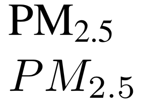
So, one simple use for custom commands is to save you typing the same thing over and over again. In my thesis I talked a lot about air quality, and particularly PM2.5. Now, the correct way to typeset that in LaTeX is as:
$\text{PM}_{\text{2.5}}$
This uses math-mode, but keeps the PM and the 2.5 as ‘normal text’ (otherwise it will look like P multiplied by M rather than PM as an abbreviation for particulate matter). This is a pain to keep typing all of the time – so a lot of people just write
$PM_{2.5}$
which looks far worse (the top is ‘right’, the bottom is ‘wrong’):
Luckily, LaTeX’s ability to create new commands really easily can be used to save us a lot of work. Adding the following to your preamble (the section of your document before the \begin{document} line) will create a new command called \pmtext which will insert the ‘proper’ version of the PM2.5 code from above:
\newcommand{\pmtext}{$\text{PM}_{\text{2.5}}$}
As you can see, \newcommand is quite simple, you give it two arguments: the name of the new command, and what the new command ‘does’. In this case the second argument is just some LaTeX code that typesets the PM text properly. I created this command fairly early on in the process of writing my PhD, and it made life a lot easier: I had less to type, I didn’t have to remember exactly how to typeset PM2.5 properly, and if I wanted to change how it was displayed I just had to change it in one place (basically all of the standard benefits of commands or functions in any programming language!).
Talking of programming languages, you can do far fancier things with \newcommand, including passing parameters. A good example here is some code that I add to every LaTeX document I write, which creates a new command called \todo. See if you can work out what it does:
Yup, that’s right: it displays the given text as bold and red – a perfect way to mark something that still needs doing. For example:
\todo{Somewhere here put in the radiosonde type boxplot}
will produce something that looks like this:
If you look at the \newcommand call, you can see that we give it an extra parameter in square brackets: this is the number of parameters that the command has. We can then reference the value of these parameters as #1 for the first parameter, #2 for the second etc. The rest of the ‘body’ of the command is just normal LaTeX code (if you want to use this code, make sure you add \usepackage{xcolor} too, so that the \textcolor command will work!).
The other command I add to almost every document I use is this:
\newcommand{\rh}{\todo{REF HERE }}
It depends on the \todo command, and allows me to mark the fact that I need to add a reference to a bit of text, without having to stop writing and actually find the reference. I find this has actually helped my writing a lot – as I can quite happily write multiple paragraphs and just scatter \rh around to remind me to come back and put in references later.
The final command I used a lot in my thesis, which shows a slightly more advanced use of \newcommand is
\newcommand\xcaption[2]{\caption[#1]{#1#2}}
You may know that the \caption command can take an optional argument in square brackets for a short caption to be used in the List of Figures. Something like
\caption[Example Landsat image over Southampton]{Example Landsat image over Southampton, shown as a true colour composite, with XYZ procedure applied. Image data from USGS.}
As in that example, I often found myself repeating bits of text: I normally wanted the short caption to be the first part of the long caption, without all of the details given in the long caption. So, the \xcaption command (‘extra caption’) command I’ve created just takes two arguments, the first of which is the short caption, and the second of which is the text to add to the short caption to get the long caption – saving a lot of typing and mistakes!
So, I hope that’s shown how easy it can be to create simple new commands in LaTeX that can save you a lot of time and effort.
In the previous part we had established that the Worcester Wave thermostat app communicates with a remote server (run by Worcester Bosch) using the XMPP protocol, with TLS encryption. However, because of the encryption we haven’t yet managed to see the actual content of any of these messages!
To decrypt the messages we need to do a man in the middle attack. In this sort of attack we put insert ourselves between the two ends of the conversation and intercept messages, decrypt them and then forward them on to the original destination. Although it is called an ‘attack’, here I am basically attacking myself – because I’m basically monitoring communications going from a phone I own through a network I own. Beware that doing this to networks that you do not own or have permission to use in this way is almost certainly illegal.
There is a good guide to setting all of this up using a tool called sslsplit, although I had to do things slightly differently as I couldn’t get sslsplit to work with the STARTTLS method used by the Worcester Wave (as you may remember from the previous part, STARTTLS is a way of starting the communication in an unencrypted manner, and then ‘turning on’ the encryption part-way through the communication).
The summary of the approach that I used is:
I configured a Linux server on my network to use Network Address Translation (NAT) – so it works almost like a router. This means that I can then set up another device on the network to use that server as a ‘gateway’, which means it will send all traffic to that server, which will then forward it on to the correct place.
I created a self-signed root certificate on the server. A root certificate is a ‘fully trusted’ certificate that can be used to trust any other certificates or keys derived from it (that explanation is probably technically wrong, but it’s conceptually right).
I installed this root certificate on a spare Android phone, connected the phone to my home wifi and configured the Linux server as the gateway. I then tested, and could access the internet fine from the phone, with all of the communications going through the server.
Now, if I use the Worcester Wave app on the phone, all of the communications will go through the server – and the phone will believe the server when it says that it is the Bosch server at the other end, because of the root certificate we installed.
Now we’ve got all of the certificates and networking stuff configured, we just need to actually decrypt the messages. As I said above, I tried using SSLSplit, but it couldn’t seem to cope with STARTTLS. I found the same with Wireshark itself, so looked for another option.
Luckily, I found a great tool called starttls-mitm which does work with STARTTLS. Even more impressively it’s barely 80 lines of Python, and so it’s very easy to understand the code. This does mean that it is less configurable than a more complex tool like SSLSplit – but that’s not a problem for me, as the tool does exactly what I want . It is even configured for XMPP by default too! (Of course, as it is written in Python I could always modify the code myself if I needed to).
So, running starttls-mitm with the appropriate command-line parameters (basically your keys, certificates etc) will print out all communications: both the unencrypted ones before the STARTTLS call, and the decrypted version of the encrypted ones after the STARTTLS call. If we then start doing something with the app while this is running, what do we get?
Well, first we get the opening logging information starttls-mitm telling us what it is doing:
LISTENER ready on port 8443 CLIENT CONNECT from: ('192.168.0.42', 57913) RELAYING
We then start getting the beginnings of the communication:
Fairly obviously, C->S are messages from the client to the server, and S->C are messages back from the server (the numbers directly afterwards are just the length of the message). These are just the initial handshaking communications for the start of XMPP communication, and aren’t particularly exciting as we saw this in Wireshark too.
The STARTTLS message is sent, and the server says PROCEED, and – crucially – starttls-mitm notices this and announces that it is ‘wrapping sockets’ (basically enabling the decryption of the communication from this point onwards).
I’ll skip the boring TLS handshaking messages now, and skip to the initialisation of the XMPP protocol itself. I’m no huge XMPP expert, but basically the iq messages are ‘info/query’ messages which are part of the handshaking process with each side saying who they are, what they support etc. This part of the communication finishes with each side announcing its ‘presence’ (remember, XMPP is originally a chat protocol, so this is the equivalent of saying you are ‘Online’ or ‘Active’ on Skype, Facebook Messenger or whatever).
It basically seems to be a HTTP GET request embedded within an XMPP message. That seems a bit strange to me – why not just use HTTP directly? – but at least it is easy to understand. The URL that is being requested also makes sense – I was on the ‘home screen’ of the app at that point, so it was grabbing the status for displaying in the user-interface (things like current temperature, set-point temperature, whether the boiler is on or not, etc).
Oh. This looks a bit more complicated, and not very easily interpretable. Lets format the main body of the message formatted a bit more nicely:
HTTP/1.0 200 OK
Content-Length: 640
Content-Type: application/json
connection: close

5EBW5RuFo7QojD4F1Uv0kOde1MbeVA46P3RDX6ZEYKaKkbLxanqVR2I8ceuQNbxkgkfzeLgg6D5ypF9jo7yGVRbR/ydf4L4MMTHxvdxBubG5HhiVqJgSc2+7iPvhcWvRZrRKBEMiz8vAsd5JleS4CoTmbN0vV7kHgO2uVeuxtN5ZDsk3/cZpxiTvvaXWlCQGOavCLe55yQqmm3zpGoNFolGPTNC1MVuk00wpf6nbS7sFaRXSmpGQeGAfGNxSxfVPhWZtWRP3/ETi1Z+ozspBO8JZRAzeP8j0fJrBe9u+kDQJNXiMkgzyWb6Il6roSBWWgwYuepGYf/dSR9YygF6lrV+iQdZdyF08ZIgcNY5g5XWtm4LdH8SO+TZpP9aocLUVR1pmFM6m19MKP+spMg8gwPm6L9YuWSvd62KA8ASIQMtWbzFB6XjanGBQpVeMLI1Uzx4wWRaRaAG5qLTda9PpGk8K6LWOxHwtsuW/CDST/hE5jXvWqfVmrceUVqHz5Qcb0sjKRU5TOYA+JNigSf0Z4CIh7xD1t7bjJf9m6Wcyys/NkwZYryoQm99J2yH2khWXyd2DRETbsynr1AWrSRlStZ5H9ghPoYTqvKvgWsyMVTxbMOht86CzoufceI2W+Rr9
So, it seems to be a standard HTTP response (200 OK), but the body looks like it is encoded somehow. I assume that the decoded body would be something like JSON or XML or something containing the various status values – but how do we decode it to get that?
I tried all sorts of things like Base64, MD5 and so on but nothing seemed to work. I gave up on this for a few days, while gently pondering it in the back of my mind. When I came back to it, I realised that the data here was probably actually encrypted, using the Access Code that comes with the Wave and the password that you set up when you first connect the Wave. Of course, to decrypt it we need to know how it was encrypted…so time to break out the next tool: a decompiler.
Yes, that’s right: to fully understand exactly what the Wave app is doing, I needed to decompile the Android app’s APK file and look at the code. I did this using the aptly named Android APK Decompiler, and got surprisingly readable Java code out of it! (I mean, it had a lot of goto statements, but at least the variables had sensible names!)
It’s difficult to explain the full details of the encryption/decryption algorithm in prose – so I’ve included the Python code I implemented to do this below. However, a brief summary is that: the main encryption is AES using ECB, with keys generated from the MD5 sums of combinations of the Access Code, the password and a ‘secret’ (a value hard-coded into the app).
def encode(s):
    abyte1 = get_md5(access + secret)
    abyte2 = get_md5(secret + password)

    key = abyte1 + abyte2

    a = AES.new(key)
    a = AES.new(key, AES.MODE_ECB)
    res = a.encrypt(s)

    encoded = base64.b64encode(res)

    return encoded

def decode(data):
    decoded = base64.b64decode(data)

    abyte1 = get_md5(access + secret)
    abyte2 = get_md5(secret + password)

    key = abyte1 + abyte2

    a = AES.new(key)
    a = AES.new(key, AES.MODE_ECB)
    res = a.decrypt(decoded)

    return res
Using these functions we can decrypt the response to the GET /ecus/rrc/uiStatus message that we saw earlier, and we get this:
It may not be immediately apparent what each field is (three character variable names – great!), but some of them are fairly obvious (CTD presumably stands for something like Current Time/Date), or can be established by decoding a number of messages with the boiler in different states (showing that DHW stands for Domestic Hot Water and BAI for Burner Active Indicator).
We’ve made a lot of progress in the second part of this guide: we’ve now decrypted the communications, and worked out how to get all of the status information that is shown on the app home screen. At this point I set up a simple temperature monitoring system to produce nice graphs of temperature over time – but I’ll leave the description of that to later in the series. In the next part (Part 3) we’re going to look at sending messages to actually change the state of the thermostat (such as setting a new temperature, or switching to manual mode), and then have a look at the Python library I’ve written to control the thermostat.
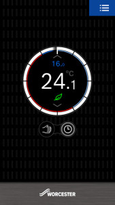
When we bought a new boiler last year, we decided to install a ‘smart thermostat’. There are a wide range available these days, including the Google Nest, the Hive (from British Gas), and the Worcester Bosch ‘Wave’. As we had a Worcester Bosch boiler we got the Wave – and it wasn’t much more expensive than a standard programmer/thermostat.
The thermostat looks like this:
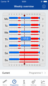
It is mounted on the wall at the bottom of our stairs, and is connected by a cable to the boiler. As you can see, it has a simple touch-sensitive interface: you can increase or decrease the thermostat setting, see the current temperature and the current setting, change from manual to program mode, and see whether the boiler is on or not. For anything more advanced (such as setting the programmable timer) you have to use the mobile app, which looks like this:
Looks familiar, doesn’t it? You have the same simple interface on the app ‘home screen’, but you can also configure the more advanced settings, such as the timer programme:
Overall, I’m pleased with the Wave thermostat: it is far easier to configure the timer settings on a phone app than on a tiny fiddly controller, and there are all sorts of advanced features you can use (for example, ‘optimisation’, where the system gradually learns how long it takes your house to warm up, and turns the heating on at the right time to get it to the temperature you want at the time you want) – combined with being able to control the heating when away from home.
Anyway, of course one of the first things that I looked for once it had been installed was an API that I could use to monitor and control the thermostat from my home server, ideally through a Python script. Unfortunately there was nothing about an API on the Worcester Bosch website, and when I phoned Customer Services they told me than there was no API available. So, I thought I’d try and reverse engineer the protocol that was used, and see if I could hack together a Python interface.
How does the system overall work?
When starting to investigate this, my a priori understanding of the system was that the app must send messages of some sort to a remote server (presumably run or controlled by Bosch), which then forwards the messages on to the thermostat itself, and vice-versa. This is because you can access the thermostat via the app wherever you are: you don’t have to be on the same wireless network. Whatever protocol or ports that are used must be ones that can reliably get through home firewalls so that the remote server can actually talk to the thermostat.
What technologies do they use?
When exploring the app I had noticed that there was a Product Information screen which showed information about the software and hardware versions, and included a button labelled Worcester Wave uses Open Source software. Tapping this shows a list of open-source packages that are used by the system, including their various license agreements. The list consisted of:
libresample – resampling of data (primarily audio, but presumably other datatypes too)
So, looking at that list suggests that the eXtensible Messaging and Presence Protocol (XMPP) is used for communication, potentially with some metadata embedded with the eXtensible Metadata Platform. The rest of the libraries aren’t very relevant to our work, but are interesting to see (I suspect the mathematical ones are for doing the maths for some of the advanced features like optimisation).
What is being sent, and where to?
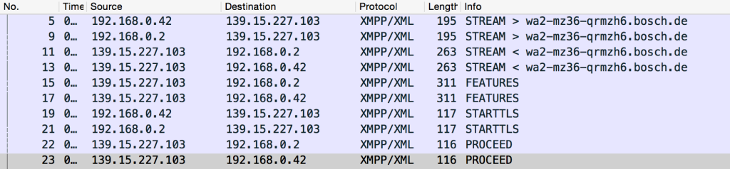
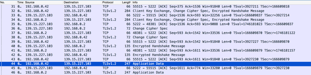
So, we think the communication is using XMPP – now we need to confirm that, and work out what is being sent and where it is being sent to. So, I opened up Wireshark to start sniffing the traffic. After playing around a bit with the filters, I got this (click to enlarge):
This shows that my guess was correct: the XMPP protocol is being used to send messages between the phone running the Wave Android app (192.168.0.42 on my local network) and a server run by Bosch (wa2-mz36-qrmzh6.bosch.de). So, we now know what protocols we are dealing with: that is the good news.
However, the bad news is the STARTTLS messages that we see there. You may recognise this from email configuration dialog boxes, as it is one of the security options for connecting to POP3/IMAP/SMTP servers. It stands for ‘Start Transport Layer Security’, and is basically a way of saying "I want to encrypt this conversation from now onwards, is that ok?" (for reference, the alternative is to do everything with encryption right from the start of the communication). Anyway, in this case the Bosch server responds with PROCEED ("Yes, I’m happy to do this encrypted"). From that point onwards, we see the TLS security negotiation ("What sort of encryption do you support?", "I support X, Y and Z", "Ok, lets use Z", "Here are my keys" etc) followed by a lot of ‘Application Data’ messages:
We can’t actually see any of the content of the messages, as they are encrypted, so all we get is the raw hex dump: 80414a90ca64968de3a0acc5eb1b50108bbc5b26973626daaa….(and so on). Not very useful!
I think this is a good place to finish Part 1 of the story. We have worked out that communication goes from the app to a Bosch server, and it uses the XMPP protocol, but with TLS encryption using STARTTLS, so we haven’t been able to work out what any of the messages actually contain. Come back for Part 2 to hear how I managed to read the messages…
My PhD was done through a Doctoral Training Centre, and as part of this I had a taught year at the beginning of my PhD. During the summer of this year I had to do a ‘Summer Project’, which was basically a MSc thesis. My thesis was called "Can a single cloud spoil the view?": modelling the effect of an isolated cumulus cloud on calculated surface solar irradiance" (I think the best thing about my thesis was the title!). It gained a ‘Distinction’ mark, and I was very pleased that it won the RSPSoc MSc thesis prize (again, I think they gave me the prize based on the title alone!). This is the story of this project…
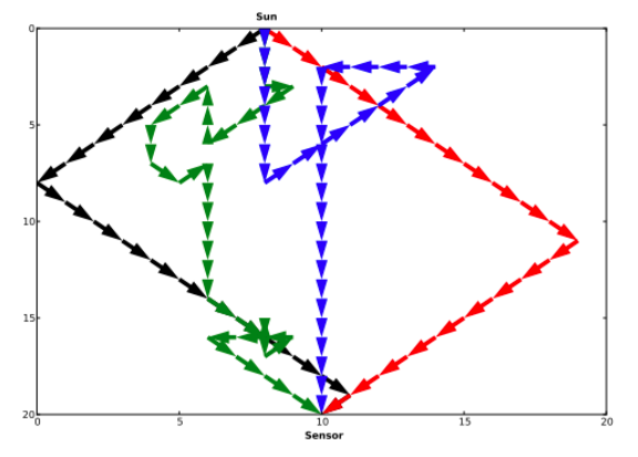
Paths taken by light in the ray-tracing Radiative Transfer Model I developed for my MSc
During the year before my MSc, I had been doing a lot of investigation into Radiative Transfer Modelling. These models (known as RTMs) are used to estimate how light travels through the atmosphere: you basically tell them what the atmosphere is like (how hazy, how much water vapour etc), and they simulate the effect on light passing through the atmosphere.
I’d investigated a range of models – including simple models like SPCTRL2, good standard models like 6S, and advanced models like SCIATRAN. One thing that I noticed was that none of these models seemed to be able to incorporate clouds very well. SCIATRAN did support modelling clouds, but you had to have either an entirely clear or entirely overcast sky – you could have vertical variation in optical properties (ie. multiple layers of clouds) but not horizontal variation. I decided that I’d write some code to use one of these RTMs to model light passing through an atmosphere which is partially cloudy and partially clear – like most of the skies that we have in the UK.
So, I started reading more about these RTMs, and tried to work out how I might be able to extend them so that I could have a spatially-variable amount of cloud (eg. cloud on the left-hand side of my ‘simulated atmosphere’ and clear sky on the right-hand side – or even a single small cloud moving across the sky). I struggled with this for a while and didn’t really have much success at working out what I’d need to do. I naively thought that I would be able to write a tiny bit of code to replace the ‘homogenous atmosphere’ that SCIATRAN used with a ‘spatially-variable atmosphere’ and that would be it. Unfortunately, that wasn’t the case…
It turns out that the horizontally-homogeneous nature of the atmosphere is a fundamental assumption of the mathematics that these models are based upon. And I’d come up with a MSc project that required me to break this assumption. Ooops.
So – after panicking a bit and deciding that I can’t do a PhD or even a MSc – I decided that if the standard models wouldn’t let me do what I wanted then I’d have to implement a new Radiative Transfer Model myself, from scratch! A bit of a tall order…but I decided to have a go, figuring that even if it didn’t work I’d learn a lot in the process.
With a bit more reading I realised that the only way to take into account horizontally-varying atmospheric properties would be to implement a ray-tracing model. In this sort of model, individual rays of light are followed from their source (the sun), and each individual interaction with the atmosphere is simulated (scattering, absorption etc). They are far more time-consuming to run than ‘standard’ models – but allow far more interesting parameterisations, as the atmosphere is basically represented by a grid, which can be ‘filled’ with different atmospheric properties in each cell. Normally the grid would be a 3D grid, but I decided to use a 2D grid to make life easier – just taking into account vertical height into the atmosphere (sun at the top, sensor at the bottom) and horizontal distance along the ground.
I decided to base my model on SPECTRL2, which meant I could use a lot of the constants that were defined in the SPECTRL2 code – for things like Earth-sun distances, absorption at different wavelengths, etc. I then built a simple Monte Carlo Ray Tracing procedure that followed the flowchart below (click to enlarge):
I say "simple" – it took quite a while to get it working properly! Of course, after actually getting the model working, I had to work out how to actually parameterise the atmosphere, how to create a realistic cloud to put in this atmosphere, and then what computational experiments to run to actually answer my original question.
Answering the actual question I set out to answer was actually very easy to do once I’d got the model running – and it gave some interesting answers. For example, if there is a cloud near a sensor on the ground, but not directly between the sensor and sun, then the sensor will actually record a higher irradiance than it would if there were no cloud. This makes perfect sense when you think about it (the cloud will scatter some extra light towards the sensor), but I hadn’t thought of it before I did the experiment!
I don’t think there’s really much more to say here, apart from to direct you to my thesis for more information (including my detailed conclusions) and to say that the code is now available on Github. I have tested the code in the latest version of IDL (v8.5) and it is still working – although I should warn you that the code runs rather slowly!
Also, if you’re interested in using a proper 3D ray tracing RTM then look into the Discrete Anisotropic Radiative Transfer Model (DART). I’ve always been meaning to replicate my experiments with DART, but have never quite had the time…that’s another thing for my ‘list of papers to publish when I have time’.
One of the most important things when developing software – particularly open-source software – is knowing when to stop working on something, relinquish responsibility and suggest that it should not be used any more. This is what I have recently done with AutoZotBib.
For those who don’t remember AutoZotBib, it is a tool that I first wrote a few years ago to automatically export Zotero bibliography libraries to the BibTeX format (used for LaTeX documents). I used it during the writing of my PhD, but there have always been some fairly significant problems with it. The main problem was performance: if you had a reasonably large Zotero library, then adding a new item would freeze the library for at least thirty seconds, while the export was performed. In fact, the Zotero developers added a warning to the plugins list page saying that my plugin may slow Zotero down significantly if you use it with a large library!
Over the years I did various updates to try and make this work better – and, in fact, I wrote most of a new version that did intelligent caching and only wrote out the bits that had changed…but I never quite got it fully working and never found the time to push it through to completion.
I haven’t had any time to work on it recently (the last commit was February 2014), and I haven’t even had the time to respond to the occasional support emails that I receive. I’d been thinking of dropping support for a while, but I wasn’t aware of anything else that did the same job, and I always had a hope that maybe, one day, I might find time to work on it.
Two things snapped me out of this, and made me accept that I needed to drop it:
The latest version of Firefox requires all plugins to be signed, and as Zotero is a Firefox plugin (although it can run in standalone mode too), any Zotero plugins will also have to be signed. I tried to get AutoZotBib signed, but a lot has changed in the Firefox extension world since I first wrote it, and I couldn’t get it to work.
I’ve found another plugin that does similar things, but does them better – and is well-maintained! It’s called Zotero Better BibTeX, and its Push Export feature does exactly what AutoZotBib did, but allows you to configure it to only export specific collections, allows export only when the computer is idle, etc.
So, I took a deep breath and updated the website to say that AutoZotBib is deprecated, and marked it as such on the Zotero Plugins page, suggesting that users use BetterBibTeX instead. Doing this has really taken a load off my mind – and I am now happy that I don’t have to try and motivate myself to work on it. Of course, the beauty of open-source software is that the code is still available, and so if anyone else wants to pick it up (or is desperate to use it, even though it is no longer supported) then they can!