I often find myself using Julian days as a simple method to represent dates in my code. It’s nice and easy, because every day is simply an integer (the number of days since the beginning of the year) and any time during the day can be represented as a floating point number (the fraction of that day which has elapsed at that point). Furthermore, lots of satellite imagery is provided with the dates specified as Julian days – for example, MODIS data filenames include the year and then the Julian day.
It’s fairly easy to convert a standard date (eg. 24th March) to the Julian day in most programming languages (there will either be a library function to do it, or it’s fairly simple to write one yourself) – but it’s not that easy to do in your head. So, I have created a Julian Day calendar poster:
It’s a very simple table that lets you choose the month and day, and get the Julian Day number. Just make sure you remember the note at the top – add one to the number (after February) if it’s a leap year!
I was helping some undergraduates with some work the other day, and they decided to use the following colour scheme for representing river depth:
Deep water: Red
Medium-depth water: Bright green
Shallow water: Pink
Why did they do this? Well, either they were the default values used by the software they were using (unlikely), or they just chose randomly. Not a good idea.
If you look you’ll find a huge amount of literature about this (I should put some references here but I can’t really be bothered at this time at night), and it really makes your maps a HUGE amount more useable if you’re using sensible colours. For example:
Deep water: Dark blue
Medium-depth water: Medium-blue
Shallow water: Light blue
Why is this sensible? Well it makes sense on a number of levels – water is normally shown as blue (so it’s obviously some kind of water), and the different levels of colour imply some sort of ordering. With the original colours above there is no inherent ordering – is green ‘higher’ or ‘lower’ than red? Of course, red and green being used for ‘incorrect’ and ‘correct’ on a different map would be very sensible…
Isn’t it hard work to come up with nice colour schemes for all of your maps? Nope not at all – ColorBrewer has done it already! If you haven’t used this website already I urge you to do so, it provides a number of carefully-chosen colour-schemes designed for various different purposes. For representing river depth you’d probably want to use one of the blue Sequential schemes, but there are also Diverging schemes for data that goes off in two directions, as well as schemes for representing Qualitative data (those that have no explicit ordering). What’s more you can tell it to only show schemes that are color-blind-friendly, photocopier-safe etc, and it’ll produce a preview for you with various map styles (labels, cities, coastlines etc). All in all it’s very impressive, and very useful.
Plugins and extensions are available for a number of pieces of software to allow ColorBrewer colours to be easily used. These include an ArcGIS plugin (see the bottom answer for how to install with ArcGIS 10), R package, Python module and IDL routines.
I’m starting a new series here on my blog about interesting and somewhat out-of-the-ordinary applications of remote sensing. So…here is number 1.
An analysis firm called Remote Sensing Metrics LLC has been using satellite images to predict changes in the profits of firms such as Walmart, and thus help predict share prices. How does this work? Well it’s fairly simply – for a firm like Walmart, the more people shop in its stores, the more profitable it will be. Of course, this is a generalisation, but there is likely to be a fairly strong correlation between these two variables. So, all you need to do is find a way to estimate how many people shop at Walmart.
How does remote sensing come into this? Well, you just use high resolution imagery and count the cars in the car parks at their stores. Obtaining base-line data for a number of stores, and then looking at the trends should give a guide to trends in profits. If you want to go further – and these analysts did – you can perform a regression to obtain a quantitative relationship between the number of cars seen in the car parks and the profits of the company.
The technicalities of the approach aren’t detailed in the article – for obvious commercial reasons – but it seems that the data is provided by sensors such as QuickBird and Geo-Eye, which have resolutions down to 40cm. This means they can easily resolve cars – which tend to be at least 1m wide by 2m long. Whether they count the cars using human analysts, or whether some sort of object-based image analysis is used to classify cars in defined areas (the selected car parks), I don’t know – but I suspect the latter.
What do you think of this? Clever use of technology, or "Cold War-style satellite surveillance" (as CNBC put it)? Why not leave a comment.
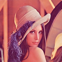
When doing a course in Computer Vision last year I was introduced to the Lena image:
This was originally a scan from Playboy magazine in 1972, but has taken on a life of its own as a test image in the field computer vision. The (very interesting) history of it is described on the Wikipedia page and in the Complete Story of Lena. The image, freely available online, has been used as a test image for a huge amount of research in computer vision including image compression, face recognition, edge detection and more. Of course, Lena isn’t the only test image used in computer vision and image processing, there are many others (see, for example, these images). The use of a standard set of test images has a number of benefits:
It allows easy comparison between methods – Statistical measures of error will be comparable as they are based on the same underlying image data. Visual comparisons by humans will also be possible.
A range of test images can be chosen which range from easy to difficult to process – Lena is a good image to use for compression tests as it has a number of areas with high detail, but also larger flat areas. The subtly varying tones of the skin are also important, particularly when dealing with compression to lower colour depths.
Everyone working in the field can have access to the same images – 30 years ago, if you didn’t have a colour scanner (which were very expensive at the time), there was little you could do to get a colour test image – but the free distribution of the Lena image changed that. Similarly now, everyone from a Professor at a top research lab to a hobbyist working in their garage can have access to the same original data and perform tests which can easily be compared with the state of the art.
Research becomes more reproducible – Using test images means that other researchers can get hold of the data used in a study, and if they either get access to the code used to produce the results, or manage to re-implement the method themselves from a description in the paper (not always easy), they can then try and reproduce the results.
So, the question is:
Why don’t we have similar test images in remote sensing?
One of the things I leant on my computer vision course is that image processing for remote sensing is actually very similar to image processing for computer vision (whether it is face recognition, checking for cracks in contact lenses or anything else). In both fields, when you’re trying to do something (for example compress a photo or classify a satellite image) there are many methods to choose from. You want to choose the best for your situation, or decide whether you need to develop a new approach, and so you need to be able to compare the approaches easily.
A simple set of test remote sensing images would allow this. Of course the major questions are:
What sort of images do we want to pick?
How on earth are we going to deal with copyright, file format and distribution issues?
The second question is probably the more difficult (although less ‘scientifically important’) question – but there are a number of possible solutions, including getting imaging companies to release a few small portions of one of their images for free, or using freely-available data such as Landsat data. File format issues shouldn’t be too difficult – providing images as ENVI .bsq files (with a header file) and ERDAS .img files should allow easy use in the most common software, and make it fairly easy to read the data manually into another filetype. As for distribution, maybe a nice friendly university could be persuaded to host a website for us…
Now, the more interesting question: what sort of images do we want to pick? As with the test images discussed above, we want to have a range of image types and a range of image ‘difficulties’. As a first guess I’d suggest something like the following:
Small segment of urban area – Interesting because of the huge range of land covers, and notoriously difficult to classify. Three resolutions (high, medium, low) would be good, allowing comparisons between results at different resolutions. Ground truth data would be brilliant, but is likely to be expensive to collect.
MERIS (300m)
Landsat (30m)
IKONOS (4m)
Airborne (0.5m)
Extended area of vegetation – useful for testing vegetation data extraction algorithms. In this case, a phenological time-series would be useful, as well as different resolutions (as above).
Mixed landscape – a mixture of land-cover types including water, vegetation, urban and others. Preferably again at a number of resolutions.
These images don’t need to be huge – whole Landsat scenes would become unwieldy and take too long to process – but they should be large enough to contain enough pixels for statistically significant model development.
The main difference between the images available for testing computer vision algorithms and the images needed for remote sensing is that remotely sensed data must have good metadata. These images must be provided with full metdata including instrument type, bands used, resolution, date/time of collection, calibration data and map reference data. Ideally data should be provided fully atmospherically and geometrically corrected.
Of course, to do this would be a lot of work – far more work than most academics (including myself) have time for – but I think it would be an important and useful resource.
What do you think? I’d love to hear some feedback.
Many fields have a collection of rules of thumb – tacit knowledge that isn’t often talked about, but is often used in the field. Some of these rules have come from published information (papers, books, presentations etc) and some has just grown up over the years.
This post isn’t anywhere near done yet – I’m going to try and keep this post up-to-date as I learn more of the rules of thumb used in Remote Sensing.
Green vegetation reflects at about 5% in the Red and 40% in the Near Infrared. This is useful for getting an approximate reflectance for vegetation from surface irradiance spectra, or for checking reflectance values gathered in the field. (Source: personal communication, E. J. Milton)
Around 40% of the radiance from a pixel comes from outside of the pixel area. This obviously varies based on the sensor and the viewing characteristics, but this seems to be a fairly good approximation for many purposes. (Sources: Various papers, for example Ruiz and Lopez (2002) for the SPOT sensor).
Calibration sites should be at least 3×3 pixels. This is also sometimes stated as the calibration site area should be at least eight times the pixel area, which is roughly equivalent. This ensures that boundary effects are not too large, and that errors in geometric correction do not affect the location of the site too much.
A spectral resolution of around 20nm is sufficient for identification of most materials found on Earth. This was discussed in a seminal article by Goetz and Calvin (1987), and means that any instrument with a spectral resolution greater than this is literally hyper-spectral – as in it gives too much data. However, this extra data can still be useful for various purposes (for example, accurately locating certain atmospheric absorption bands)
10-100 training pixels are required per class for accurate Maximum Likelihood classification. This was discussed in Swain and Davis (1978) and is generally taken to be a useful approximate guess.
3 arc-second resolution is approximately 90m resolution. Not much more to say really – although of course remember that the size of an arc-second in metres varies across the globe.
References:
Goetz, A. and Calvin, W., 1988, Imaging spectrometry – Spectral resolution and analytical identification of spectral features, in Society of Photo-Optical Instrumentation Engineers (SPIE) Conference Series, 834, 158-165
Ruiz, C.P. and Lopez, F.J.A., 2002, Restoring SPOT images using PSF-derived deconvolution filters, International Journal of Remote Sensing, 23(12), 2379-2391
Swain, P.H. and Davis, S.M., 1978, Remote sensing: The quantitative approach, McGraw-Hill, New York, 405pp
As part of the OS Open Data initiative the Ordnance Survey has released a free version of their 1:50,000 scale gazetteer. This lists all of the names shown on the 1:50,000 scale OS maps, linked to information such as their location (in both Ordnance Survey grid references and WGS84 latitude/longitude pairs) and type (city, town, water feature etc). I’ve had a little play with this data to do some statistics on it and see if I can find out anything interesting. Hopefully you’ll agree that at least some of the stuff below is interesting.
My main statistical analysis was to count the frequency of each name in the gazetteer, and then extract the ten most commonly-used names for each of the feature types listed in the database.
Cities: No cities in the UK share a name with another city.
Towns:
There are 1,245 towns in the dataset and the results here are slightly more interesting – the winner is Seaton, of which there are three (in Cornwall, Devon and Yorkshire). This isn’t particularly surprising as Seaton was probably derived from Sea Town, and given that we are an island nation, there is a lot of sea by which towns could be located! A number of names are well-known for belonging to two towns in the UK, such as Newport, St. Ives and Ashford, but there are 12 such towns, listed below:
Armadale
Ashford
Gillingham
Heathfield
Newport
Ramsey
Richmond
Rothwell
Royston
Slough
St Ives
Swinton
Other settlements: This is where it starts to get more interesting, but also more confusing. The feature type of Other Settlements seems to include anything that’s not a town or a city and there are over 34,000 of them. Nearly 31,000 of these are unique (a fairly impressive feat), but a number of them seem to be more popular than the rest – the top ten are listed below and include three variations on calling a place a new town (New Town, Newtown and Newton) as well as a number of other names relating the settlements to their location (West End, North End, East End) or what is there (Church End).
Newtown
55
West End
49
Newton
48
Church End
42
North End
36
New Town
32
Upton
32
Milton
30
East End
28
Mount Pleasant
26
I was intrigued by the differences between the names of New Town, Newtown and Newton and wondered if there may be differences across the country in which name was used. Also, I wondered whether any areas of the country had significantly more of these new settlements than others. The map below shows the distribution of the three names across the country (click to see a larger version):
A number of patterns are noticeable:
There seem to be a lot of these settlements around the Welsh border (the area known as the Welsh Marches). I’d suspect this is because of the frequently changing location of the border in this area, leading both sides to rename a town as ‘new’ once they’d captured (or re-captured) it.
There is a distinct lack of these settlements in central Wales – fairly obviously, as most names there are in Welsh
Scotland has far more Newtons than any other version of the name, and these are concentrated on the eastern side of the country.
New town seems to be far more common in southern England, although there is a concentration of Newtons in Cornwall.
I’m not sure what exactly one can learn from the above, but it’s interesting to me at least. If anyone has any ideas which explain the distribution of these names better then leave a comment.
1. Conference presentations are not like undergraduate lectures In an undergraduate lecture you go in, listen to someone talk for a long time, and try and write down/remember as much of it as possible – because almost any of it could come up on the exam. It was not uncommon for me to have 3-4 pages of handwritten notes for a 45 minute lecture. Conferences aren’t like that – you don’t need to remember (or even understand!) all of the details and you only need to care about the bits you actually care about. Why is this? Well, you’re not going to be examined on it, and you can get the details from the author another way (through the paper in the conference proceedings or via email etc). Most importantly though – you only need to be interested in the stuff that is interesting or useful to you – now you’re a researcher no-one else is telling you what to be interested in, you have to decide that yourself!
I first noticed this during some departmental seminars where I was taking notes and so was my supervisor, who was sitting next to me. During the seminar I took about 2 pages of notes, and my supervisor wrote about 5 words. I had treated the seminar like a lecture, and tried to get down all of the information – he had focussed on just the bits that were really interesting to him.
I must admit I still find this very difficult – four years of lectures have got me into the ‘write everything’ mindset, but I tried hard to be more selective at this conference, and I think I did fairly well. I tried to make notes on the bottom of the page in the conference booklet that showed the abstract for the presentation – which could be quite hard if the abstract was long!
2. Show your interest in other people’s work People want you to be interested in their work – if you get excited about it they’ll be excited too, they won’t label you as a ‘geek’ or ‘weird’. In fact, nothing seems to make researchers happier than having a really in-depth conversation about their work with someone who is really interested.
3. Show your interest in your work – all the time No matter who you are talking to, show how interested and excited you are about your work, and how great you think it is. Why? Well, hopefully you are interested in your work, but also – you never know who you’re talking to. I spoke to someone who I thought was ‘just an academic’, turned out he was in charge of funding for the majority of my field in my country. My excitement in my project and explanation of why I think it is important may have paid off…
4. Social events are important We had a lot of nice social events at this conference (including a boat trip around Poole harbour and a very nice meal at a fancy hotel). Most of the really interesting conversations I had were during these events – whether they were learning about the academic environment in different countries, discussing research projects, or coming up with really bad remote sensing jokes. Getting to know people in the social events gets you known amongst the community, so next time someone sees your name as an author they remember you – always useful.
I’ve just discovered something that I feel I must share here – partly to make more people aware of it, and partly so I don’t forget it. In the IDL programming language you will sometimes find your program interrupted by a line saying something like:
% Program caused arithmetic error: Floating divide by 0
Sometimes it will be obvious where the error is – but often you can spend ages looking for it (just like with segfaults in C…). What I only just found out is that if you run the command
!EXCEPT=2
At the IDL prompt before running your program you will get a far more informative error message like
% Program caused arithmetic error: Floating divide by 0
% Detected at JUNK 3 junk.pro
The key thing is that this tells you what line the error occurred on (line 3 of junk.pro in the above example) – which helps you to narrow down the problem far more quickly.
More details on the values that !EXCEPT can take is available here – basically the options are no messages, unhelpful messages and helpful messages.
This is very useful – but just beware that running with !EXCEPT=2 all the time will slow down your code, so only do it if you need to for debugging purposes.
If you use iPython, particularly if you do work with matplotlib or with parallel programming, you should use the latest release.
It. Is. Great.
For those who don’t know, iPython is a replacement console for Python that offers many improvements over the standard console. For example, everything has tab completion, syntax highlighting is available, there are many magic commands (eg. %run, %edit etc), you can run standard terminal commands simply by adding ! to the beginning (eg. !wget www.google.com) and much more. With the latest (admittedly still unstable) release there are two major new features:
Parallel Programming support – you can create a team of python worker processes which can then be, very easily, set tasks to do. It even has support for automatic load-balancing (something which even some very fancy parallel programming environments can’t do!). As nearly all computers are multicore these days, and as many scientists have access to fairly sophisticated supercomputers, this is a great step for Python
GUI console – you can now use iPython in a GUI. So what? you ask – I like the terminal! Well, I like the terminal too, but having a GUI means two things:
Tooltips – as soon as you type a function name and an open bracket a tooltip will pop up giving you the list of parameters for the function and the doc-string (or at least as much of as it which will fit).
Embedding of graphics – yes, now you can embed plots from matplotlib in your console just like Matlab or Mathematica users can. What’s more, you can also export the whole console session (with both the figures and the text) to a HTML file – great for teaching use (I’m already planning how I can do this…)
iPython was always great – now it’s even better!
For more details please see here, and follow SciPyTip on Twitter to get regular tips and news for SciPy users.
I haven’t had chance to try it yet, but I’m wondering whether libraries like the Python Imaging Library or Spectral Python will also be able to put figures directly into the iPython GUI terminal. Maybe I need to work on some integration for those – that’d be great for my remote sensing teaching!
As part of my research I do a fair amount of data collection in the field. Some of the instruments I use are very modern and connect to a computer via USB, interacting with custom-written client software which allows such luxuries as timed logging, triggered logging and local calibration. However, a number of the instruments are older and don’t have computer-based logging capability, requiring you to log data to their internal memory and then download it later.
This is often perfectly satisfactory, but timing can be an issue. For example, when taking measurements using a number of instruments it is often important to make sure that measurements are taken at the same time. For example, if spectral measurements are being taken and other instruments (for example sunshine sensors, like the sensor shown below) are being used to gather data which can then be used to atmospherically correct the spectra, then it is very important to ensure that measurements are taken at the same time. This is particularly a problem in areas of fast changing weather like the UK, where sky conditions can change very quickly.
A tool called SJinn allows you to send simple strings over a RS-232 (standard serial port) connection and then obtain data sent back by the instruments. One of the examples given by SJinn is the following:
rs232 -b600 -p7n2 -s"\n" -r16
This sends a newline character over the serial port (at 600 baud with 7 data bits and 2 stop bits) and then returns the next 16 characters send on the line. In this case, it would provide the voltage measured by a digital voltmeter. As this is simply a command-line tool, it is very easy to combine into scripts, and thus use to collect timed measurements (eg. via the use of the cron daemon). I have used similar techniques to obtain measurements from the sunshine sensor shown above – a script for which will be available on my website soon.
 It’s a very simple table that lets you choose the month and day, and get the Julian Day number. Just make sure you remember the note at the top – add one to the number (after February) if it’s a leap year!