I don’t seem to have time or energy for long posts these days, but here’s another quick post which might save you some time and frustration.
Recently, I’ve been trying to import OpenStreetMap data into a PostGIS database to use with pgRouting. I wanted to import data for the whole of England – which has quite a lot of roads!
I initially tried following standard guides online, to do roughly the following:
This takes the england_latest.osm file, uses a config for cars (so it doesn’t try to route down paths, but only routes that are accessible to cars), specifies how to connect to the database, what schema to use and what prefix to use.
I tried running this and it ran for hours and hours and eventually crashed with loads of errors of the form:
While processing FROM 1800000th          to: 1820000th way
count1820000 While processing FROM 1800000th     to: 1820000th way
[********************|                              ] (40%) Total processed: 1840000
ERROR:  relation "__ways8380" does not exist
I eventually worked out that the way to solve this is to add a --chunk 10000000 parameter to the command line call. This is a big increase on the default chunk size, and has two benefits:
It stops it crashing – which is always good!
It massively speeds up the import, taking it from running for many hours (and then failing) to finishing successfully in about 45mins
I’m not entirely sure how the larger chunk size stops the crash, but the speedup seems to come because osm2pgrouting uses the Postgres COPY command (which is very efficient), and with a larger chunk size it runs the COPY command a few times with large chunks of data rather than loads of times with small chunks of data.
Warning: You will need a computer with a lot of RAM to run this successfully with a large chunk size. I used a temporary cloud VM with a large amount of RAM which only cost me about £5.
A Discord server I use has a channel called #til, standing for Today I Learned. It’s a place to post interesting or surprising things you recently learned.
I took my posts to that channel from the last couple of years, tidied them up and have listed them below. Hopefully you’ll find something interesting there:
TIL that elements with even atomic numbers are more abundant than elements with odd atomic numbers, because of the way elements are formed through fusion. [Source]
TIL that the BCG vaccine (for TB, you may have had it as a child/teenager) is also an effective chemotherapy treatment for bladder cancer, apparently by causing a local immune reaction against the tumor. [Source]
TIL how guns are traced by serial numbers in the US, with no computers allowed. [Source]
TIL a lot about the extremely complex engineering behind the Manhattan Project. [Source]
TIL more details about how various types of display screens work. [Source]
TIL that by freezing (literally, lowering the temperature significantly) a RAM chip, you can keep the values there for a while after removing power, allowing attackers to extract chips and read them [Source]
TIL that when replacing some ball-and-socket joints, surgeons will sometimes reverse the joint when the natural socket is badly damaged. [Source]
TIL that the British Library was only created in 1973 as a combination of several earlier libraries, including the British Museum Library. [Source]
TIL that a PDF of the first issue of Linux Format magazine (from 2000) is available online, featuring distributions like Mandrake and Corel Linux. [Source]
TIL how much the UK National Lottery was played in the 1990s, with around two-thirds of adults buying tickets weekly, despite extremely poor odds. [Source]
TIL about the Volkswagen sausage — a genuine VW product with an official part number. [Source]
TIL that UK police operate at least one fixed-wing aircraft as well as helicopters (and when I learned this it was circling over my house). [Source]
TIL that in 1841, the population of Ireland was 8.2 million, more than three times that of Scotland, and over half that of England. Then the potato blight came. There are still fewer people living on the island of Ireland than there were in 1841. I knew the Irish potato famine was bad, but I hadn’t realised the population had never grown back to the levels before it. [Source]
TIL that the processor name Pentium comes from pent meaning five — effectively the successor to the 486 (i.e. 586).
TIL that pyrophones are musical instruments that produce sound via explosions or rapid heating, described as “internal combustion instruments.” [Source]
TIL that Plymouth has roughly double the population of Exeter – for some reason I thought Exeter was larger. [Source][Source]
TIL about the enormous complexity involved in building and operating semiconductor fabrication plants. [Source]
TIL that datacentres consumed 18% of Ireland’s electricity in 2021–22, and likely more since. [Source]
TIL that there is a place in England called New Invention, with debate over what the invention actually was. [Source]
TIL about the surprisingly varied cow silhouettes used on European road signs. [Source]
TIL about the idea that “the rain follows the plough,” a mistake of correlation for causation suggesting that starting to farm desert/dry lands will bring rain [Source]
TIL that a radio station for biscuit-factory employees became Britain’s first independent radio station. [Source]
TIL about unusual and humorous units of measurement. [Source][Source]
TIL that apparently I had completely the wrong idea about belly dancing. I assumed you danced on your belly, but apparently the thing I was picturing was breakdancing. [Source]
I really haven’t got much time or energy at the moment (I spent most of the Christmas break with an extremely painful back, which was exhausting and frustrating), but I wanted to post a very brief list of books I read this year. I read a total of 44 books this year, which includes re-reads and audiobooks. A lot of them aren’t included here as they’ve been included in other lists I’ve posted, or are childrens books I’ve been re-reading.
The books listed below have a significant tech/nerd/infrastructure focus, but cover a fairly broad set of fields even so. I hope you find something interesting to add to your ‘to read’ list!
Killing Thatcher – About the attempted assassination of Thatcher by the IRA. Fascinating in general, covers a lot of Irish/British history, police approaches, IRA structures and so on. I learned a lot, was shocked by a lot, and thoroughly enjoyed reading it.
A Brush with Steam: David Shepherd’s Railway Story – Very good, lots of stuff about how the early steam preservation movement got going, plus crazy tales of African railways in the 60s. Remarkably funny in places, with absurd BR bureaucracy and things falling off the back of lorries.
Concorde – One of the best Concorde books I’ve read, with a load of stuff that was new to me.
The Boy Who Played with Fusion – I read The Radioactive Boy Scout last year, and found it really depressing. This is a far happier book, and still interesting.
Fuelling the Wars: PLUTO and the Secret Pipeline Network 1936–2015 – Very good; fascinating the way the oil pipeline network in the UK developed over the years, and the amount of infrastructure involved. Something I knew barely anything about before, but I’m now pointing out ‘pipeline posts’ to my wife when driving down country roads!
Petroleum Refining in Nontechnical Language – Bits of it were a bit above me (I only did chemistry to GCSE level), but it gave me a far better idea of what goes on at the oil refinery near us (Fawley, on the shore of Southampton Water).
A Classless Society: Britain in the 1990s by Alwyn W. Turner – a fascinating tour through the 1990s in Britain, covering everything from politics and law to popular culture. As someone who lived through the decade but didn’t really pay attention to the wider world (I was still a young child), it was fascinating.
I’ve got into a bit of a habit of writing occasional posts with links to interesting things I’ve found (probably because it’s a relatively easy blog post to write). This is another of those posts – this time, written in June 2025. So, let’s get on with some links:
Why COUNT(*) can be slow in Postgres: a good delve into how Postgres works ‘under the hood’ and why that means that counting rows can sometimes be quite time-consuming
f2: handy command-line tool for bulk-renaming files, with the default mode being a dry-run
Leaflet v2.0 alpha: an alpha version of a new major version of Leaflet, the web mapping library. I actually tend to use MapLibre these days (it seems faster for MVTs, though I haven’t tested that properly), but I prefer the Leaflet API and tend to use it for simpler applications. The new version seems to tidy up a lot of stuff, which is good.
cqlalchemy: this is a handy library (named after SQLAlchemy and almost impossible to pronounce in a way that makes clear it is different) for writing Common Query Language queries, as used with many STAC catalogs. It’s a right pain to write these queries by hand, and they often have to be structured weirdly in JSON, but this library will do it all for you.
stac-fastapi-geoparquet: this is a backend for the stac-fastapi tool (a STAC server written in FastAPI) that lets you store the STAC catalog in GeoParquet rather than in the standard options of a Postgres database (via pgstac) or ElasticSearch. Storing STAC information in GeoParquet files is something I’ve been keeping an eye on for a while, and there are some interesting talks on it – like this one.
stac-auth-proxy: One final STAC-related link, this time an authentication proxy to run a private, secured STAC server. This is something I implemented a proof of concept of myself with a previous client, and it’s nice to see there’s something ‘off the shelf’ for it now.
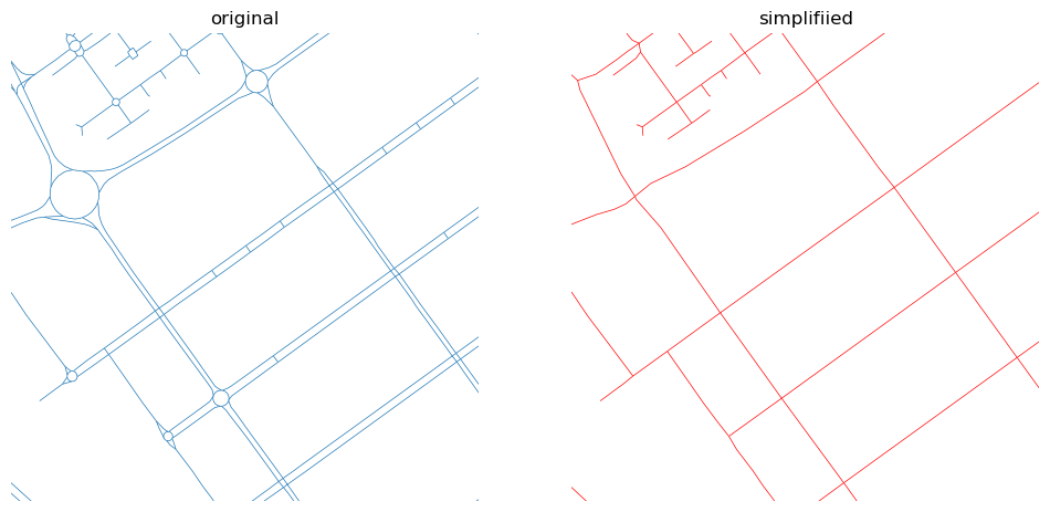
Simplification of street networks: A nice description of a Python tool to simplify street networks, removing things like sliproads, roundabouts and so on, and just leaving the correct topology there. It’s quite a nice tool, but also a nice approach to solving the problem.
Promptfoo: This looks like a good tool for evaluating AI model responses – easily configurable, open-source etc. There’s a good description of the tool and links to other resources on Simon’s blog. Another interesting post on evals for AI model responses is here.
Adding notes to exceptions in Python: a brief post explaining a new feature in Python 3.11 which allows you to add handy notes to exceptions – I could see this being useful for some more complex errors in some of my libraries
How to get auto-complete to automatically appear in pgAdmin: I’m not a massive fan of pgAdmin, but I’ve tried a range of Postgres GUIs and haven’t really found one I like more (yet…). This little change to the settings in pgAdmin will make it pop up the autocomplete dropdown when writing SQL queries just while you’re typing, rather than waiting for you to press a key combination – making everything a little bit smoother.
Design for 3D printing: I’ve been getting quite into 3D printing recently (I’m hoping to write a post on it soon), and this is a great, very detailed, article on how to design items ready for 3D printing. I learnt a lot!
llm can run tools now: Simon’s llm command-line tool and Python library can now use the ‘tool usage’ pattern with local tools defined very easily as Python functions. Seems very powerful, and a lot simpler than some other approaches.
I recently gave a careers talk to students at Solent University, and through that I got to know a MSc student there who had previous GIS experience and was now doing a Data Analytics and AI MSc course. Her GIS experience was mostly in the ESRI stack (ArcGIS and related tools) and she was keen to learn other tools and how to combine her new Python and data knowledge with her previous GIS knowledge. I wrote her a long email with links to loads of resources and, with her permission, I’m publishing it here as it may be useful to others. The general focus is on the tools I use, which are mostly Python-focused, but also on becoming familiar with a range of tools rather than using tools from just one ecosystem (like ESRI). I hope it is useful to you.
Tools to investigate:
GDAL
GDAL is a library that consists of two parts GDAL and OGR. It provides ways to read and write geospatial data formats like shapefile, geopackage, GeoJSON, GeoTIFF etc – both raster (GDAL) and vector (OGR). It has a load of command-line tools like gdal_translate, ogr2ogr, gdalwarp and so on. These are extremely useful for converting between formats, importing data to databases, doing basic processing etc. It will be very useful for you to become familiar with the GDAL command-line tools. It comes with a Python interface which is a bit of a pain to use, and there are nicer libraries that are easier for using GDAL functionality from Python. A good tutorial for the command-line tools is at https://courses.spatialthoughts.com/gdal-tools.html
Command line tools in general
Getting familiar with running things from the command-line (Command Prompt on Windows) is very useful. On Windows I suggest installing ‘Windows Terminal’ (https://apps.microsoft.com/detail/9n0dx20hk701?hl=en-GB&gl=GB) and using that – but make sure you select standard command prompt not Powershell when you open a terminal using it.
GeoPandas – like pandas but including geometry columns for geospatial information. Try the geopandas explore() method, which will do an automatic webmap of a GeoPandas GeoDataFrame (like you did manually with Folium, but automatically)
rasterio – a nice wrapper around GDAL functionality that lets you easily load/manipulate/save raster geospatial data
fiona – a similar wrapper for vector data in GDAL/OGR
shapely – a library for representing vector geometries in Python – used by fiona, GeoPandas etc
rasterstats – a library for doing ‘zonal statistics’ – ie. getting raster values within a polygon, at a point etc
Conference talks
These can be a really good way to get a brief intro to a topic, to know where to delve in deeper later. I often put them on and half-listen while I’m doing something else, and then switch to focusing on them fully if they get particularly interesting. There are loads of links here, don’t feel like you have to look at them all!
FOSS4G conference YouTube videos:https://www.youtube.com/@FOSS4G/videos – they have a load of ones from 2022 at the top for some reason, but if you scroll down a long way you can find 2023 and 2024 stuff. Actually, better is to use this playlist of talks from the 2023 global conference: https://www.youtube.com/playlist?list=PLqa06jy1NEM2Kna9Gt_LDKZHv1dl4xUoZ
Here’s a few talks that might be particularly interesting/relevant to you, in no particular order
Suggestions for learning projects/tasks (These are quite closely related to the MSc project that this student might be doing, but are probably useful for people generally)
I know when you’re starting off it is hard to work out what sort of things to do to develop your skills. One thing that is really useful is to become a bit of a ‘tool polyglot’, so you can do the same task in various tools depending on what makes sense in the circumstances.
I’ve listed a couple of tasks below. I’d suggest trying to complete them in a few ways:
Using QGIS and clicking around in the GUI
Using Python libraries like geopandas, rasterio and so on
Using PostGIS
(Possibly – not essential) Using the QGIS command-line, or model builder or similar
Download OS data on buildings from this page – https://automaticknowledge.org/gb/ – you can download it for a specific local authority area
Find all buildings at risk of flooding, and provide a count of buildings at risk and a map of buildings at risk (static map or web map)
Extension task: also provide a total ground area of buildings at risk
Task 2 – Elevation data
(Don’t do this with PostGIS as its raster functionality isn’t great, but you could probably do all of this with GDAL command-line tools if you wanted)
Mosaic the tiles together into one large image file
Do some basic processing on the DEM data. For example, try:
a) Subtracting the minimum value, so the lowest elevation comes out as a value of zero
b) Running a smoothing algorithm across the DEM to remove noise
I did a post a while back which was just a lot of links to things I found interesting, mostly in the geospatial/data/programming sphere. Since then I’ve collected a lot more links – so here are some of them. The theme, such as there is, seems to be ‘this would have really helped me about X contracts ago, if it had existed then/I had known about it then’. Make of that what you will…
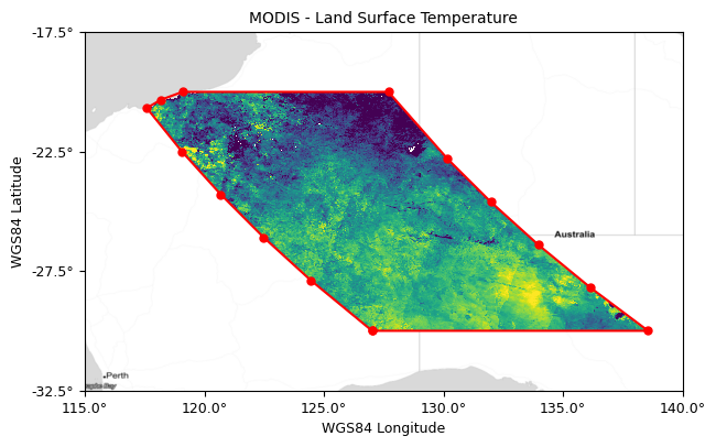
The stac-tools raster footprint utility – a useful new-ish tool that generates nice, accurate but simple outlines (‘footprints’) for the area covered by a raster file (as shown above) all ready to put into a STAC catalog
Is Antarctica Greening? – a brief article looking at some of the technicalities of using NDVI time series to monitor greening in Antarctica (reminds me of some of the issues I had using time series in my PhD)
VTracer – an interactive web interface to an open-source tool to convert raster images to vector SVGs (not geospatial images, just images in general). Gives great immediate feedback on parameter changes
tilegroxy – a proxy that can sit between end users of web map raster/vector tiles and the sources, managing things like caching, authentication etc. Seriously considering using this with my current client.
grid-banger – a Python package for converting between Ordnance Survey grid co-ordinates and latitude/longitude. Unlike many converters, it works with both fully numerical grid references, and those that start with letters (like TQ213455)
GeoDeep – a new and simple (but seemingly quite powerful) tool for doing basic deep learning on geospatial rasters. Can do things like extract cars, trees, buildings – and even extract road polygons (something which would have been useful a couple of clients ago…)
LosslessCut – not geospatial or data related, but very useful: I’ve recently been digitising some old VHS tapes, and this makes it very easy to mark chunks of video files and then export each chunk to a separate file – all while keeping the quality high
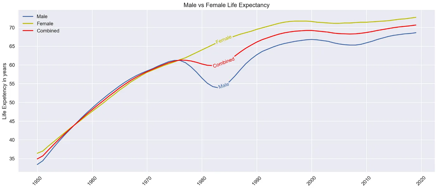
labellines – a neat little Python package for labelling lines on a graph by putting the label inside the line, rather than relying on a separate legend (see image below)
act – lets you run Github Actions locally, to save doing a million commits to see how your CI/deployment/etc runs. This would have saved me a lot of time about four contracts ago.
cuttle – this one isn’t even tech related, it’s the rules for a fairly fun card game that I’ve been playing with my wife recently. Sometime I’ll do a blog post containing my player cheatsheet that I put together.
It’s cool to care – a blog post from Alex Chan where they explain something that is very important to me: that it is cool to be enthusiastic/interested/excited by something, even if other people aren’t.
FILTER in Postgres – simple explanation of a nice bit of SQL syntax in Postgres that allows you to write things like SELECT COUNT(*) FILTER (WHERE b > 11)
QMapCompare plugin for QGIS – a useful plugin that lets you compare two views of a map, either side-by-side, with a swipe or with a focus area following the map
BGNix – a 100% free way to remove backgrounds from images (again, not geospatial in this case – just things like photos or clipart). It uses an AI model that runs entirely on your local device, and so doesn’t send your images anywhere making it high-privacy too!
Spy for changes with sys.monitoring – nice example of how to use the new sys.monitoring functionality (a newer, better version of sys.settrace) in Python to help with debugging
QGIS Deepness – a plugin for easily running deep learning models in QGIS, including a ‘model zoo’ of models that can be set up very quickly
lonboard – I mentioned lonboard in my last list of links – it’s a Python library for creating interactive maps – but hugely faster than most alternatives. Here’s a new version with animation added, allowing some pretty cool animated maps to be made.
geopandas – another new release, this time for geopandas with some nice new functionality
As always, this post is very delayed – apologies. In fact, I was encouraged to write this by a friend who I see at PyData Southampton (Hi, if you’re reading this!). I mentioned my talk in passing to her, and she asked if I’d blogged about it yet. I admitted that I hadn’t, and promised I would by the next PyData Southampton. Well, I totally failed at that – but there is another PyData Southampton meetup on Tuesday, so I’m going to get it done in time for that.
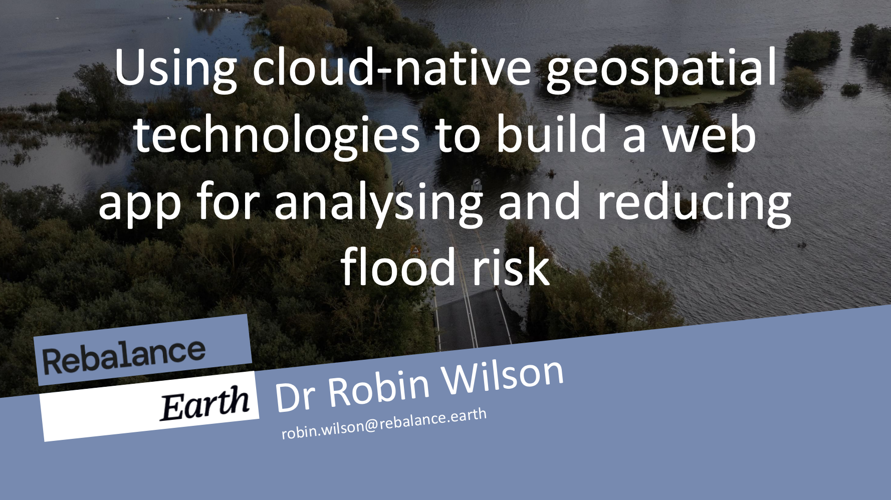
The FOSS4G UK South West conference 2024 took place in Bristol on 12th November. I gave a talk there entitled Using cloud-native geospatial technologies to build a web app for analysing and reducing flood risk, talking about some of the work I’ve done with the company I’m currently working with: Rebalance Earth.
The talk covers the development of a web app for looking at assets (businesses, buildings, substations etc) that are at risk from flooding in the UK, and comparing various flood scenarios to understand how risk could be reduced by Natural Flood Management strategies such as river restoration. After introducing Rebalance Earth and the web app itself, I talk about the technologies behind it and the ‘cloud native’ manner in which it was designed. I specifically cover generating Mapbox Vector Tiles on-the-fly from a PostGIS database, and generating raster tiles on-the-fly from COG files stored in cloud storage.
Full slides are available here. There is also a video recording of the talk available, but it’s a bit hard to watch as you can’t see the slides on the video.
Once you’ve had a look at my talk, don’t forget to check out the other talks that were given at the conference, they were great!
I just shared this approach with some friends, and thought I’d blog it here too.
When I get a relatively small amount of monetary compensation for something, I take the ‘Feynman Approach’ to it and buy something fun with the money, giving me a sense of satisfaction from the compensation (which, presumably, was to compensate me for something bad that happened).
Now, it’s some dopey legal thing, but when you give the patent to the government, the document you sign is not a legal document unless there’s some exchange, so the paper I signed said,
"For the sum of one dollar, I, Richard P. Feynman, give this idea to the government . . ."
I sign the paper.
"Where’s my dollar?"
…[he eventually gets the dollar]
I take the dollar, and I realize what I’m going to do. I go down to the grocery store, and I buy a dollar’s worth – which was pretty good, then – of cookies and goodies, those chocolate goodies with marshmallow inside, a whole lot of stuff.
I come back to the theoretical laboratory, and I give them out: "I got a prize, everybody! Have a cookie! I got a prize! A dollar for my patent! I got a dollar for my patent!"
…[everyone else wants to get a real dollar for their patent]
I don’t usually spend the compensation amount on sweets or baked goods (unless it’s really quite small), but I often buy myself a little something I wanted for fun – like a few electrical components, a 3D printing accessory (or filament), or just a second-hand book (or a new one if the amount is enough).
Recent bits of compensation I’ve used this approach with are mostly Delay Repay for delayed trains (it means I was inconvenienced by the train delay, so I ‘deserve’ something nice), but it can apply to other things too. I don’t usually apply it if the compensation is reasonably large, and obviously not if I’m really short of money (in that case the money goes into ‘general funds’), but for compensation less than £15-20 it’s often an approach I take.
(I should point out that I definitely don’t agree with Feynman on everything, particularly some of his views on women, but in general I enjoyed his books)
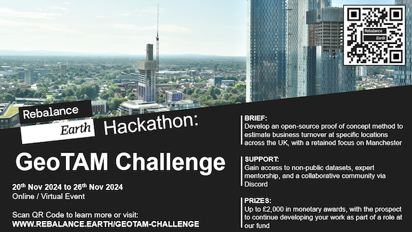
Summary: I’m involved in organising a hackathon, and I’d love you to take part. The open-source GeoTAM hackathon focuses on estimating turnover for individual business locations in the UK, from a variety of open datasets. Please checkout the hackathon page and sign up. There are prizes of up to £2,000!
(Click image for a larger version)
I’m currently working with Rebalance Earth, a boutique asset manager who are focused on making nature an investable asset. Our aim is to mobilise investment in UK natural infrastructure – for example, by arranging investment to undertake river restoration and reduce the risk of flooding. We will do this by finding businesses at risk of flooding, designing restoration schemes that will reduce this risk, and setting up ‘Nature-as-a-Service’ contracts with businesses to pay for the restoration.
I’m the Lead Geospatial Developer at Rebalance Earth, and am leading the development of our Geospatial Predictive Analytics Platform (GPAP), which helps us assess businesses at risk of flooding and design schemes to reduce this flooding.
An important part of deciding which areas to focus on is estimating the total business value at risk from flooding. A good way of establishing this is to use an estimate of the business turnover. However, there are no openly-available datasets showing business turnover in the UK – which is where the hackathon comes in.
We’re looking for participants to bring their expertise in programming, data science, machine learning and more to take some datasets we provide, combine them with other open data and try and estimate turnover. Specifically, we’re interested in turnover of individual business locations – for example, the turnover of a specific supermarket, not the whole supermarket chain.
The hackathon runs from 20th – 26th November 2024. We’ll provide some datasets, some ideas, and a Discord server to communicate through. We’d like you to bring your expertise and see what you can produce. This is a tricky task, and we’re not expecting fully polished solutions; proof-of-concept solutions are absolutely fine. You can enter as a team or an individual.
Most importantly, there are prizes:
£2,000 for the First Prize
£1,000 for the Second Prize
£500 for the Third Prize
and there’s a possibility that we might even hire you to continue work on your idea!
A quick post today to talk about a couple of PostGIS functions I learnt recently.
I had a CSV file that contained well-known binary (WKB) representations of geometries, stored as hexadecimal strings. I imported the CSV into a PostGIS database, and wanted to convert these to be proper PostGIS geometries.
I initially went for the ST_GeomFromWKB function, but kept getting an error that the function didn’t exist. Well, actually the error said that it couldn’t find a function that exists with that name and those specific parameter types. That’s because I was calling it with the text column containing the hex strings, and the documentation for ST_GeomFromWKB says that its signature is one of:
So, we need to convert the hexadecimal string to a bytea type – that is, a proper set of bytes. We can do this using the decode function, which takes two parameters: the text to decode, and a format specifier which must be one of base64, escape or hex. In this case, we’re decoding a hex string, so we want the latter.
Putting this together, we can write some simple SQL that does what we want. First, we create a geom column in our table:
ALTER TABLE test ADD geom Geometry;
and then we set that column to be the result of decoding the hex and converting the WKB to a geometry:
UPDATE test SET geom = ST_GeomFromWKB(decode(wkb_column, 'hex'), 4326);
Note that here I knew that my WKB was encoding a point in the WGS84 latitude/longitude co-ordinate system, so I passed the EPSG code 4326 which refers to this co-ordinate system.