UPDATE: I’ve created a new site to host my John Snow data, and included various other modern formats (GeoPackage, GeoJSON etc). Please go there to download the data.
In honour of the bicentenary of John Snow’s birth – and because I was asked to by someone via email – I have now released my digitisation of John Snow’s Cholera data in a few other formats: KML and as Google Fusion Tables.
To save you reading my previousblog posts on the subject, I’ll give a brief overview of my data. John Snow produced a famous map in 1854 showing the deaths caused by a cholera outbreak in Soho, London, and the locations of water pumps in the area. By doing this he found there was a significant clustering of the deaths around a certain pump – and removing the handle of the pump stopped the outbreak. This is a bit of a simplification (see Wikipedia or the John Snow Society for more details), but generally covers what happened.
These are available for download/use in a number of formats:
A zip file with the Vector data as Shapefiles and the Raster data as TIFF images
(this is the original data provided for download by me – and is probably what you want for importing into a GIS system) Download
A zip file with the Vector data as KML files and the Raster data as TIFF images
(suitable for importing into Google Earth and other products that use KML files) Download
Links to Google Fusion Tables with the vector data already imported Cholera Deaths Pumps Deaths and Pumps together (this dataset has both pump and death points in the same table: pump points have Count values of -999, death points have Count values > 0 which give the number of Cholera deaths at that location)
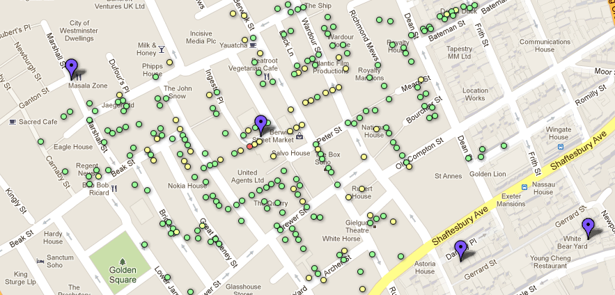
The latter is particularly cool, I think as it allows you to very easily overlay the data on modern Google Maps data, and should allow some interesting ‘mashups’ to be created. All of the tables are set to be shared publically, so you could be able to copy them (using the Copy Table command in the File menu) and play around with them as much as you want! If you click the Example Map tab then you’ll see a very rudimentary map I’ve created using the data on top of Google Maps (see below) – I’m sure you’ll be able to do far better visualisations than that.
The folks at CartoDB have also used this data in one of their tutorials which shows you how to import the data to CartoDB and create a styled map to show the deaths with different sized markers – yet another way you can use the ‘first real GIS data’ in today’s modern web-based GIS tools.
So, enjoy – and please let me know (via the comments below) what you create!
Update: There was a problem with the KML files and Google Fusion Tables that I uploaded yesterday, caused by an incorrect co-ordinate transformation between the Ordnance Survey grid references and latitude/longitude. This has now been fixed and the downloads and tables have been updated. Sorry about this.
I recently did a presentation entitled Sustainable Software and Reproducible Research in Remote Sensing at the Wavelength 2013 conference. The slides are available at SpeakerDeck, and shown below.
The rest of this page is a rather rough categorised list of various links and resources that may be useful to you after seeing the presentation (either in person at the conference, or online).
My blog posts
I’ve looked at some of these issues before on this blog. The most relevant posts are:
Saleska, Scott R., et al. “Amazon forests green-up during 2005 drought.”Science 318.5850 (2007): 612-612. PDF
Samanta, Arindam, et al. “Amazon forests did not green-up during the 2005 drought.” Geophysical Research Letters 37.5 (2010): L05401. PDF
Irish, Richard R., et al. “Characterization of the Landsat-7 ETM+ automated cloud-cover assessment (ACCA) algorithm.” Photogrammetric engineering and remote sensing 72.10 (2006): 1179. PDF
Tang, Jiakui, et al. “Aerosol optical thickness determination by exploiting the synergy of TERRA and AQUA MODIS.” Remote Sensing of Environment 94.3 (2005): 327-334. PDF
Aruliah, D. A., et al. “Best Practices for Scientific Computing.” arXiv preprint arXiv:1210.0530 (2012). PDF
Sustainable Coding
This is basically just good coding practices. Various resources are relevant:
Software Carpentry – look under Lessons for online lessons on various things (automated testing, version control, documentation, debugging, code program structure etc) and Boot Camps to see if there is a training day coming up near you.
Code Complete (2nd Edition) – a big book with loads of information on good coding styles etc. Your library is likely to have a copy
Version Control by Example – a great book by Eric Sink (disclosure: I proof-read it for him and gave various bits of feedback, and therefore got a free copy) which covers the concepts of version control in general, and then shows how they apply to various real-world systems such as Git, Mercurial and Subversion.
Science Code Manifesto – a manifesto for how software and code should be treated in science.
Remote-Sensing-related:
ArcGIS has a number of tools and functions that make it easier to do reproducible research.
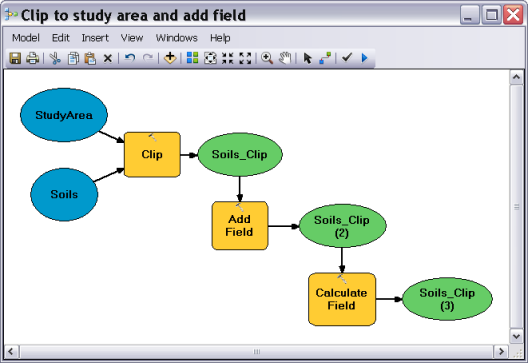
Model Builder is a great way to get started with automating your ArcGIS analyses without having to learn to program. It allows you to build an automatic workflow through drag-and-drop, and is really handy for automating things you do frequently, for documenting your processes and more. It can even export your models to Python code, so you can start bridging the gap between Model Builder and full Python programming. For more information look at the documentation, or Google for tutorials. (Similar tools exist in a number of other pieces of software, including Idrisi – but unfortunately not ENVI – although if you have the ArcGIS ENVI toolbox installed you can use many ENVI tools from ArcGIS).
Example of ArcGIS Model Builder
My ArcGIS Provenance tool is not yet working well enough to be released, but until it is, you can look at your history manually (its hard to understand that way, but better than nothing). See my blog post about ArcGIS logs here XXX
ENVI
ENVI can be scripted in IDL, but it is generally harder than ArcGIS scripting in Python – details are on the ENVI website in the ENVI Programmers Guide. At the time of writing (March 2013), I would strongly suggest using the ENVI Classic IDL API, rather than the modern API for ENVI 5.0 onwards, as the latter is not really finished yet.
ENVI also had a log system (turn it on under File->XXX). The logs it produces are easier to read by hand than those created by ArcGIS, but harder for a computer to read…
If you are developing some sort of method/algorithm which works on satellite data to produce an output, publishing the results generated from a freely-available input image (eg. MODIS, Landsat etc) allows others to verify their work when they try and reimplement your method.
If you are collecting field spectra, please try and collect metadata along with it – fulfilling the requirements of: H, Andreas, et al. “Metadata of spectral data collections.” 5th EARSeL Workshop on Imaging Spectroscopy, Bruges, Belgium. 2007. PDF
General Reproducible Research
Tools
All of the tools below are available to use today – so have a go, try them out, and see what happens. The only tool which isn’t available is something called Burrito. It is described in an article by its author who wrote it as part of his PhD. It was only a prototype and requires some rather unusual system settings (for example, Linux with an entirely different filesystem) – but it really shows the sort of things we should aim for in terms of reproducible research tools.
Gloo – same idea as ProjectTemplate, but for Python
Repro – a build-tool-based approach for automating scientific computation
Sumatra – tracking and documentation tool for scientific computation
VCR – Verifiable Computational Research, a tool to allow you to store and verify computer-based research.
Useful sites
Lots of people online have come up with useful tutorials, guides and discussions about reproducible research – some of them say that they are about other fields, but lots of ideas are easily transferrable between fields.
How to define Reproducible Research – This is a more philosophical discussion of what Reproducible Research actually is – whether being able to click a button and run the computations again is all that is needed, or whether there is more to it than that.
General Sustainability
The Software Sustainability Institute do lots of work on software sustainability, but also cover data sustainability, and work with Software Carpentry
Software Carpentry have various online lessons, and also run boot camps, all of which teach good scientific software development practices.
Updated 6th Jan 2020: This post has been updated to fix the code example and the link to the Landsat shapefile download.
As part of some work I was doing for my PhD, I needed to automatically find what Landsat scene path and row would contain a pixel with a certain latitude/longitude co-ordinate (this was basically so I could automatically download the relevant Landsat image and do some processing on it).
There is an online converter (provided by the USGS) which allows you to input latitude/longitude and get back path/row, but it doesn’t have an API of any kind, and I couldn’t see an easy to way to automatically submit requests to the form, as they’ve (very sensibly really) included methods to stop people doing that.
Summary: So, I wrote my own code to do the conversion. It’s available on Github and depends on GDAL/OGR and Shapely. See the README file on Github for instructions.
Very helpfully, the USGS have made shapefiles of the WRS-2 scene boundaries available to download, so all my code needs to do is load the shapefile, do some ‘Point in Polygon’ operations to find out which polygon(s) the point is in, and extract the ‘path’ and ‘row’ attributes from those polygons. This is fairly easy to do in Python using the wonderful OGR library to access shapefiles, and Shapely to do the ‘Point in Polygon’ operations. When writing this I used the Python Geospatial Development book as a good reference for how to combine GDAL and Shapely in this way.
The code is available at GitHub, with instructions on how to install it (basically, download the shapefiles from the USGS – I’m deliberately not re-distributing them here – and download the Python script), and it is very easy to use:
Instantiating the class may take a while, as it has to load in the shapefile
The get_wrs method may return multiple results, as Landsat scenes overlap at all four edges.
Please let me know (via a comment on this post) if you find this code useful.
For reference, the code is shown below, and is well-commented to show how it works:
import ogr
import shapely.geometry
import shapely.wkt

class ConvertToWRS:
    """Class which performs conversion between latitude/longitude co-ordinates
    and Landsat WRS-2 paths and rows.
    Requirements:
    * OGR (in the GDAL suite)
    * Shapely
    * Landsat WRS-2 Path/Row Shapefiles - download from USGS site
     (http://landsat.usgs.gov/tools_wrs-2_shapefile.php), you want wrs2_descending.zip
    Usage:
    1. Create an instance of the class:

        conv = ConvertToWRS()
    (This will take a while to run, as it loads
    the shapefiles in to memory)
    2. Use the get_wrs method to do a conversion:
        print conv.get_wrs(50.14, -1.43)
    For example:
        >>> conv = ConvertToWRS()
        >>> conv.get_wrs(50.14, -1.7)
        [{'path': 202, 'row': 25}]
        >>> conv.get_wrs(50.14, -1.43)
        [{'path': 201, 'row': 25}, {'path': 202, 'row': 25}]
    """
    def __init__(self, shapefile="./wrs2_descending.shp"):
        """Create a new instance of the ConvertToWRS class,
        and load the shapefiles into memory.
        If it can't find the shapefile then specify the path
        using the shapefile keyword - but it should work if the
        shapefile is in the same directory.
        """
        # Open the shapefile
        self.shapefile = ogr.Open(shapefile)
        # Get the only layer within it
        self.layer = self.shapefile.GetLayer(0)

        self.polygons = []

        # For each feature in the layer
        for i in range(self.layer.GetFeatureCount()):
            # Get the feature, and its path and row attributes
            feature = self.layer.GetFeature(i)
            path = feature['PATH']
            row = feature['ROW']

            # Get the geometry into a Shapely-compatible
            # format by converting to Well-known Text (Wkt)
            # and importing that into shapely
            geom = feature.GetGeometryRef()
            shape = shapely.wkt.loads(geom.ExportToWkt())

            # Store the shape and the path/row values
            # in a list so we can search it easily later
            self.polygons.append((shape, path, row))

    def get_wrs(self, lat, lon):
        """Get the Landsat WRS-2 path and row for the given
        latitude and longitude co-ordinates.
        Returns a list of dicts, as some points will be in the
        overlap between two (or more) landsat scene areas:
        [{path: 202, row: 26}, {path:186, row=7}]
        """

        # Create a point with the given latitude
        # and longitude (NB: the arguments are lon, lat
        # not lat, lon)
        pt = shapely.geometry.Point(lon, lat)
        res = []
        # Iterate through every polgon
        for poly in self.polygons:
            # If the point is within the polygon then
            # append the current path/row to the results
            # list
            if pt.within(poly[0]):
                res.append({'path': poly[1], 'row': poly[2]})

        # Return the results list to the user
        return res
I’m a big fan of Matt Might’s blog, and thought I’d implement one of his tips for blogging as an academic – namely Reply to Public. I’ve had a number of emails from Py6S users asking me questions about how to atmospherically-correct entire satellite images with Py6S – so I thought ‘d respond online, so that in the future people either find this response without needing to email me (ideally), or at the very least, I can point them to this blog post when they do email me.
Unfortunately, the simple answer to the question is: Py6S cannot (yet!) atmospherically correct satellite images – at least, not in a sensible manner – so I’d suggest using other atmospheric correction software such as ATCOR or FLAASH. The longer answer is below…
If you read the Py6S documentation you’ll find that there is an atmospheric correction option which you can use to take an at-sensor radiance (often called a Top of Atmosphere radiance when you’re dealing with satellite sensors) and atmospherically-correct it to get a corrected surface reflectance (or radiance) value. You could write some code to do that – it might look a bit like this:
from Py6S import *
# Create a SixS object called s
# (used as the standard name by convention)
s = SixS()

# Set the atmospheric conditions as usual
s.aero_profile = AeroProfile.PredefinedType(AeroProfile.Maritime)
s.aot550 = 0.05
s.atmos_profile = AtmosProfile.UserWaterAndOzone(2, 0.318)

# Set the wavelength
s.wavelength=Wavelength(PredefinedWavelengths.MODIS_B6)

# Set the altitudes
s.altitudes.set_target_sea_level()
s.altitudes.set_sensor_satellite_level()

# Set the geometry
s.geometry = Geometry.User()
s.geometry.solar_z= 35.8
s.geometry.solar_a= 149.4
s.geometry.view_z= 5.1
s.geometry.view_a= 106.8
s.geometry.month=06
s.geometry.date=28

# Turn on atmospheric correction mode and set it to do the
# correction assuming a Lambertian surface with a TOA
# radiance of 137.5 W/m^2
s.atmos_corr = AtmosCorr.AtmosCorrLambertianFromRadiance(137.5)

# Run the model
s.run()

# Print the result of the atmospheric correction
# (assuming Lambertian reflectance)
# This is the ground-reflectance for the given radiance,
# under the given atmospheric conditions
print s.outputs.atmos_corrected_reflectance_lambertian
This works fine, and so you might think that all you need to do to correct a satellite image is to take the code above, and run it for each pixel of the image using a for loop, as in the pseudo-code below:
# Load in the image (eg. using GDAL)

for pixel in image:
    reflectance = run_py6s(various, parameters, here)

    # Store reflectance in the output image

# Save output image
Unfortunately, that won’t work very well. Or rather, it will work – it’ll just take a long time! Let’s do some maths to work out roughly how long:
As a rough approximation, it takes Py6S around two seconds to atmospherically correct a single pixel in a single band (the exact time depends on how complicated the parameterisation is – for example, a full manual AERONET-based aerosol parameterisation will take longer than a standard aerosol model)
A full Landsat scene is roughly 5500 x 6000 pixels (170km x 185km), which is around 33 million pixels
33 million pixels x 2 seconds per pixel = 66 million seconds, or 763 days!
If I started running this now – on one band of a Landsat scene – it’d be finished around April 2015. Even if I used a simple parameterisation that only took one second per pixel, it’d still take over a year!
Now, I suspect you’re now thinking the Py6S is really awful because it takes such a long time. Well, unfortunately it’s not down to Py6S (if it was, I could try and improve it!). In fact, the Python bit of Py6S adds very little time – the vast majority of the time is taken by 6S itself.
So, maybe it’s 6S that is rubbish. Well, again, unfortunately not, or we could switch to something that is better. All other Radiative Transfer Models, such as MODTRAN, SCIATRAN etc, suffer from the same problem.
So, how on earth do people manage to correct satellite images? Obviously people have managed to do it – and there is commercial software available to do it. Well, they use something called a Lookup Table (LUT). This involves running the Radiative Transfer Model many times to produce a table of results, and then looking up the result you want in this table. Creating the table takes a long time (but nowhere near as long as 763 days!) and it often takes a lot of space to store the resulting table (for example, the Lookup Table used in ATCOR is a multi-Gigabyte file), but once you’ve got the table you can correct a pixel in a tiny fraction of a second – rather than one or two seconds – which means the correction of an image is a lot quicker.
A lookup table is a good example of two standard trade-offs in computing:
Setup time vs Run time: Often algorithms can either be designed to have a very short (or no) setup time, but then take a long time to run; or they can be designed to have a long setup phase, and then run very quickly from then onwards. Often the decision of which one to focus on depends on how often you’re going to run your process – if you want to run it multiple times (like an atmospheric correction algorithm) then it is normally better to have a long setup time (which you only have to do once!) and then a short run time.
Memory vs Time: Again, algorithms often trade speed against memory – a fast algorithm normally requires more memory, and vice-versa. In this case, a Lookup Table trades speed for memory – we have to store the Lookup Table in memory, but once we have access to it, we can do corrections very fast.
I haven’t written any code to use Py6S to create a lookup table and then use that to correct an image (although I will almost certainly write some code to do this sometime during my PhD) – but it wouldn’t be too difficult to do. The procedure would be something like the following:
Setup Phase:
Come up with a list of parameter values for all of the important parameters – choosing a number of parameters across their realistic range (there is a trade-off between accuracy and speed here, as always). For example maybe: AOT = [0.1, 0.2, 0.3, 0.4, 0.5]; solar_z = [10, 20, 30, 40, 50]; radiance = [10, 20, 30, 40, 50, 60, 70] etc.
Write some code to loop over all of these lists and run every possible combination of them
Store the result of all of these runs of Py6S (ie. the atmospherically-corrected reflectance) and the parameters used to get the result in a big table of some sort.
Correction Phase:
Loop through every pixel in the image, and for each pixel:
Get the parameters (AOT, angles, radiance etc) for that pixel
Choose the nearest parameters that were used to create results in the table (for ALL of the parameters you used)
Interpolate between these parameters as needed (eg. for an AOT of 0.15, get the results for an AOT of 0.1 and and AOT of 0.2 and interpolate) to get an interpolated ground reflectance.
Store this reflectance in another image.
This basic procedure has been used in almost all atmospheric correction tools for the last thirty years, and is described in various papers including Fraser et al. (1992) and Liang et al. (1997). Another way to speed-up the computation even more is by introducing parallel computation. If we can assume that each pixel’s atmospheric correction is entirely independent from every other pixel’s (which may not be the case in the real-world, but is generally assumed by most atmospheric correction algorithms) then we can split the pixels between a number of processors and thus correct many pixels in parallel – which gets an even greater speedup as we can do this both when generating the LUT, and when correcting the image.
Unfortunately, actually implementing this is a bit more complicated than I’ve explained here and various decisions have to be taken (including what ranges of parameters to use, how to interpolate, how best to store the multi-dimensional lookup table and more…) – but it is definitely on my ‘to do’ list as part of my PhD, and as part of Py6S.
So, in conclusion: Py6S can’t do atmospheric correction of satellite imagery in a sensible time at the moment, but should be able to within the next few years. In the meantime, I suggest using other atmospheric correction software (most of which, unfortunately, is commercial software). You may think that not being able to do this makes Py6S useless…but, as my next post will show, Py6S is still very useful for remote-sensing research.
References
Fallah-Adl, Hassan, et al. "Fast algorithms for removing atmospheric effects from satellite images." Computational Science & Engineering, IEEE 3.2 (1996): 66-77.
Fraser, R. S., Ferrare, R. A., Kaufman, Y. J., Markham, B. L., & Mattoo, S. (1992). Algorithm for atmospheric corrections of aircraft and satellite imagery.International Journal of Remote Sensing, 13(3), 541-557.
Liang, Shunlin, et al. "An operational atmospheric correction algorithm for Landsat Thematic Mapper imagery over the land." Journal of Geophysical Research 102.D14 (1997): 17173-17.
Version 1.2 of Py6S has recently been released (including a couple of bug fix releases, taking the most recent version to v1.2.2), and the major new feature in this version is the ability to use any spectrum as the ground reflectance for a model run. Previously, users were restricted to using the built-in 6S ground spectra (vegetation, clear water, lake water and sand) or doing some complicated parameterisation to set the user-defined reflectances up in the correct manner – so complicated that it was almost never worth doing!
Luckily, that has all changed in this version – read on to find out more…
Setting the Ground Reflectance
Setting the ground reflectance parameterisation in Py6S is very simple – you just use one of the methods of the GroundReflectance class. For example, to create a 6S model and set a constant reflectance of 0.5 for all wavelengths, simply run:
from Py6S import *
s = SixS()
s.ground_reflectance = GroundReflectance.HomogeneousLambertian(0.5)
s.run()
A two-dimensional array containing wavelengths (column 0, in micrometres) and reflectance values (column 1, as a fraction). This array will then be taken by Py6S, resampled to 2.5nm, subset to only the range of wavelengths being used for the current simulation, and used with the underlying 6S model.
This saves a lot of time and extra code, compared to doing all of the resampling yourself and using the user-defined spectrum option which was always available in Py6S. However, there are more benefits than this… Py6S will store the whole spectrum that you give, and just re-sample it to the correct wavelength range every time you run the model, which means you can use the lovely helper methods like run_vnirand run_landsat_tmto run simulations for a spectrum for a number of wavelengths with very little code. For example:
from Py6S import *
s = SixS()
# Somehow generate a 2D array called spectrum_array here
s.ground_reflectance = GroundReflectance.HomogeneousLambertian(spectrum_array)
wavelengths, results = SixSHelpers.Wavelengths.run_vnir(s, output_name="apparent_radiance")
Getting spectral data
Of course, that example won’t work until we add in some code to generate this 2D array for us. There are a two ways we could get this array:
Generate it within our code somehow – for example, using a simple model, or interpolation between some hard-coded values.
Load it from some sort of external datafile, for example from a CSV file using np.loadtxt
Both of those are ways that you might want to use, but I’ve added functions to Py6S to simplify a couple of ways of doing this that may be useful to people.
Firstly, the functions in the Spectra module make it easy to import spectra from the USGS Spectral Library and the ASTER Spectral Library. These two libraries seem to be the most commonly used – as far as I am aware, at least – and have a very wide range of spectra in them. The two functions are very simple to use – you simply pass the URL or file path to the spectrum data file, and it returns the right sort of array. Thus you can do:
(Either of the URLs could be replaced with a simple local file path instead, which is particularly useful if you have downloaded the USGS Spectral Library archive file, or obtained the CD of the ASTER Spectral Library).
The other way to get data is to use a model. Many models can produce spectral data, and most will output in a format like CSV that can be imported into a NumPy array really easily – but to make things even easier I have also released a Python interface to the ProSAIL called – you guessed it – PyProSAIL. Again, the methods have been carefully designed to return the right sort of arrays, so you can simply do:
# Make sure you have both PyProSAIL and Py6S installed
import pyprosail
from Py6S import *

spectrum = pyprosail.run(1.5, 40, 8, 0, 0.01, 0.009, 1, 3, 0.01, 30, 0, 10, 0, pyprosail.Planophile)
s = SixS()
s.ground_reflectance = GroundReflectance.HomogeneousLambertian(spectrum)
s.run()
So, hopefully that has been a useful introduction to how to use user-defined spectra with Py6S. I’ll leave you with an example of how to put all of this together to do something useful – that is, to run a Py6S simulation with the ground reflectance set to the spectra from every USGS spectral library file in a directory, and store the results:
from Py6S import *
import glob
import numpy as np

# Create the SixS model and set some parameters
s = SixS()
s.aero_profile = AeroProfile.PredefinedType(AeroProfile.NoAerosols)
s.altitudes.set_sensor_satellite_level()
s.altitudes.set_target_sea_level()

# Get a list of files that have the extension .asc
# (the extension used by the USGS spectral library files)
files = glob.glob("./USGSSpecLib/Selected/*.asc")

results = []

# Run the model using each filename as the ground reflectance spectrum
# using the Landsat ETM+ bands
for filename in files:
    s.ground_reflectance = GroundReflectance.HomogeneousLambertian(Spectra.import_from_usgs(filename))
    wvs, res = SixSHelpers.Wavelengths.run_landsat_etm(s, output_name='apparent_radiance')
    results.append(res)

# Stack all of the results into an array
results_arr = np.vstack(results)

# Write the results out to a CSV file for further analysis
np.savetxt("results.csv", results_arr, delimeter=",")
Another exciting update for this new year: my first academic journal paper has been published!
It’s called Py6S: A Python interface to the 6S Radiative Transfer Model, and is published in Computers and Geosciences. If you’re reading this from a university with a subscription to Computers and Geosciences then you can read it at ScienceDirect – if you don’t, then you can read the post-peer-review (but pre-publisher-typsetting) version at my website.
The paper describes the Py6S python module that I wrote to assist me in running simulations using the Second Simulation of the Satellite Signal in the Solar Spectrum (6S) model, and is fairly short, but – I hope – fairly useful. It also gives a good way for people to cite Py6S when (if…) they use it in their work – they simply cite this paper.
Of course, the issue with journal papers is that they are static – indeed, a number of things changed in Py6S during the time between submitting the paper and it coming out in print (which was around nine months!). None of those affected the example code given in the paper – and to be honest, they were mostly bugfixes – but there are some new features gradually working their way into the code.
I’m planning to start a series of posts about Py6S on this blog, showing how various things work ‘under the hood’, announcing new features, and showing examples of how to use Py6S well. Hopefully this will be useful for me and also useful for other people who may be interested in using Py6s, but may require a bit of help.
So… stay tuned for the next post which will be on a new feature involving user-defined spectra.
The New Year is a time of new beginnings – and so it is rather appropriate to launch the complete redesign of my Free GIS Data list today.
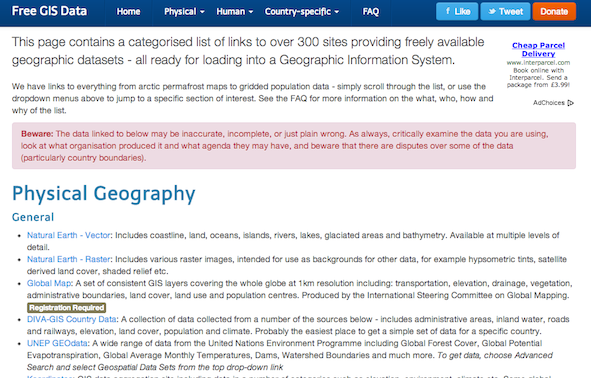
As you can see from the screenshot above, it looks far nicer than before – but it is also far easier to navigate. The dropdown menus at the top allow easy access to all of the categories (and also, incidentally, make it easier for me to add new categories as needed). I’ve also added quite a few new datasets, and tidied up some of the descriptions and categorisations of links that were already there.
Doing the re-design was around an evening’s work – mainly because I used the wonderful Bootstrap framework for the page. There were a few niggles I had to sort out (particularly regarding the header bar sticking at the top when you scroll down, and what that does for within-page anchors) but generally it was a fairly painless experience.
So, I hope the list is useful to you during 2013 and beyond!
Summary: This book takes you all the way from Morse Code to a fully working computer, explaining everything along the way. What’s more, it’s a great read too! If you ever wondered how a computer worked then buy this and read it – even if you think you already know (unless you’re, you know, a chip designer at Intel or something!)
Reference: Petzold, C., 2000, Code: The Hidden Language of Computer Hardware and Software, Microsoft Press, 395pp
As you’ll probably know if you’ve read many articles on this site: I’m a computer programmer and general ‘geek’. So, it won’t surprise you to know that I am quite interested in how computers work – and picked up this book thinking that I’d already know quite a lot of it. I knew a fair bit – but I learnt a huge amount from reading it, and it helped me gain a full understanding of what is going on when I write computer programs – right down to the level of the electricity inside the processor. By the end of the book I was itching to buy lots of relays or transformers and make a computer on my living room table!
The book starts by looking at the ways you, as a child, might try and communicate with your best friend who lives across the street – after your parents think you’ve gone to bed. The natural solution to this is Morse code using a torch, and Petzold takes this simple code as a good starting point to explain the concepts of a code. He then moves on to Braille, which is significantly more complex than I thought, and which gives the opportunity to look at some of the more complex things you find in codes (eg. shift characters and escape characters – both of which Braille has). You’ll note that nothing about computers has been introduced yet – and that is a key feature of the first part of the book, it doesn’t go straight in to "this is how a computer works", it starts at a very basic (but still interesting) level that becomes useful when thinking about computers later in the book, but isn’t too scary.
Electricity and electrical circuits are introduced when describing how you might communicate with another friend whose window you can’t see from yours. This is introduced almost entirely from scratch – explaining how circuits work, what voltage is, how batteries work etc – but it actually went beyond my previous knowledge in electricity fairly quickly, and taught me much of interest. Whenever circuits are drawn in the book – from here onwards – they are shown with the wires that have current in them in red, making it very easy to see what is going on.
The discussion of electricity for sending messages leads into the history of telegraph networks, and then the concept of relays. I’d never really understood relays before, but Petzold introduces them with a very good analogy as a ‘labour saving device’ at a telegraph station. Around this point a number of other key – but rather unrelated – topics are covered like Boolean logic (True/False, AND, OR etc) and number systems (particularly number bases and binary). There is a very practical emphasis on everything – and the point about the importance of binary as on/off, true/false, open/closed and so on, is very much emphasised. After these introductions, the relays discussed earlier are combined to produce logic gates (AND, OR, NOT, NAND, XOR and so on) with the aim of producing a circuit to help you choose a cat (yes, it sounds strange, but works well as an example!). Here you can start to see how this is moving towards a computer…
I’m not going to go much further into detail about the rest of the book, except to say that you move towards being able to ‘build’ (conceptually if not actually physically) a fully-working computer gradually, one step at a time. From logic gates, to adding circuits and subtracting circuits and from clocks to flip-flops and RAM you gradually work up to a full, programmable computer which you have basically built by page 260! Given how much detail everything is explained in – and how little knowledge is assumed – fitting it into 260 pages is very impressive!
Of course, the book continues past page 260, going on to cover topics including input and output (from keyboards and to the screen), high and low level programming languages, graphics, multimedia and more. Interestingly, transistors aren’t mentioned until after you’ve got almost all of the way to building a computer – but this is almost certainly because relays are far easier to understand, and accomplish the same job. Once they have been introduced, a couple of important processors (the Intel 8080 and the Motorola 6800) are examined in detail – a really interesting opportunity to see how the concepts you’ve learnt about have been applied in real life by chip designers.
I can think of very few issues with this book – although the last chapter does read rather strangely, as if the author was trying to fit far too much into far too little space (trying to cover multimedia, networking, WIMP interfaces and more in one chapter is a bit of a tall order though!), but I very much like the book as a whole. It is one of those rare books that is suitable for a very wide range of audiences – from those with almost no knowledge of the subject at all (it starts from the very beginning, so that isn’t a problem) right up to those who are experienced programmers and know some of it (they will still find a lot they don’t know, and realise a lot of things). Overall: a great read, very interesting and very educational. You won’t be disappointed.
So, I’ve been pondering an interesting scientific dilemma recently: how do you validate a validation technique? That is, if you’re using a certain procedure to validate some data (that is, check how correct/accurate it is), how can you validate the validation procedure itself?
This has come up in my work recently in relation to validating Aerosol Optical Thickness (AOT) data from satellites. Validation is normally performed by comparing satellite-derived data to data from the Aerosol Robotic Network (AERONET). However, this is challenging for a number of reasons: the main one being that AERONET measurements are point measurements of the AOT above the measurement site, whereas the satellite will measure AOT averaged over a large pixel area (10 x 10km for MODIS). A number of validation methods have been proposed to deal with this, and they are all based on spatial and temporal averaging of the data, to bring it into a comparable state.
Example MODIS AOT data for Europe
The big question then becomes:
If there are a number of different methods for validating this data, then how do we choose which one is best?
This is a big problem because the results of the validation will be used to infer the accuracy and uncertainty of the dataset – and if we use a validation that gives misleading results then we will have a misleading opinion of the dataset. This gets even more difficult when you need to choose parameter values for use in these validation procedures. For example, if the validation involves temporal or spatial averaging then what period/distance should the averaging be done over? 30 minutes? 1 hour? 5 hours?
So, how should we deal with this?
Unfortunately, I don’t know. I know that I have a problem with some of the current methods (for example, trying a wide range of parameter values and choosing the ones that give you the best validation results – that is, the lowest error) as some of them really do seem to be ‘cheating the system’. This is something that I’m hoping to come back to over time – I already have some preliminary ideas on how to ‘fix’ the AOT validation system – but I think it is a problem which won’t go away.
UPDATE: I’ve created a new site to host my John Snow data, and included various other modern formats (GeoPackage, GeoJSON etc). Please go there to download the data.
A while back I released a GIS dataset containing Snow’s Cholera analysis data in modern GIS formats, and georeferenced to the British National Grid (see my previous post). Unfortunately, there was an error in some of the attributes of the Cholera Deaths shapefile which caused issues when using the data.
This error has now been fixed, and the updated data are available to download here: SnowGIS_v2.zip. The link on the previous post has also been updated.
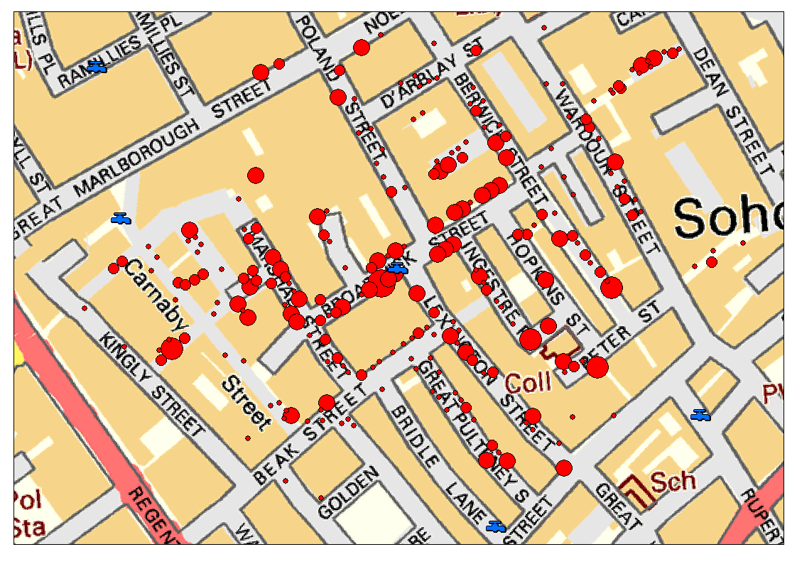
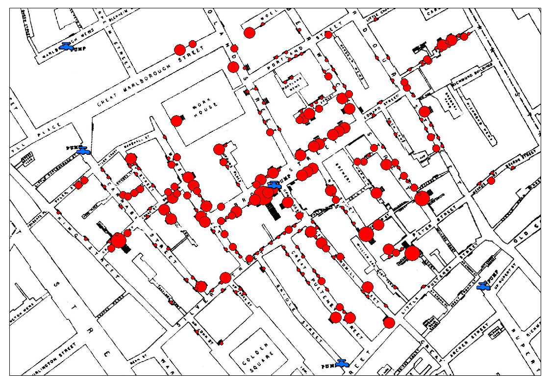 Anyway, the data that is available is: