I was looking through my past blog posts recently, and thought a few of them were worth ‘reblogging’ so that more people could see them (now that my blog posts are getting more readers). So, here are a few posts on matplotlib tips.
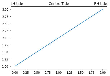
Matplotlib titles have configurable locations – and you can have more than one at once!
This post explains how to create matplotlib titles in various locations.
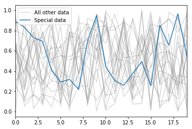
Easily hiding items from the legend in matplotlib
This post explains how to easily hide items from the legend in matplotlib.
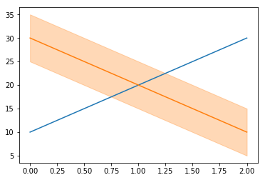
Easily specifying colours from the default colour cycle in matplotlib
This post shows how to specify colours from the default colour cycle – ranging from a very simple way to more complex methods that might work in other situations.
Recently I was interviewed on the Geomob podcast. You can listen on the Geomob site or using the embedded player below:
In the episode I talk about the British Placename Mapper and its inspiration, how I built it, and what might come next. I also cover some of my other geospatial projects including the Free GIS Data site.
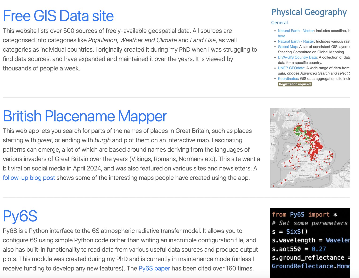
Just a quick post here to say that I’ve added a new Projects page to my freelance website. I realised I didn’t have anywhere online that I could point people to that had links to all of the ‘non-work’ (maybe that should be ‘non-paid’) projects I’ve made.
These projects include my Free GIS Data site, the British Placename Mapper, Py6S and more. I’ve also put together a separate page (linked from the projects page) with all my university theses (PhD, MSc and undergraduate) and other university work – which still get a remarkably high number of downloads.
Have a look here, or see a screenshot of the first few entries below:
I had a need to do some segmentation of some satellite imagery the other day, for a client. Years ago I was quite experienced at doing segmentation and classification using eCognition but that was using the university’s license, and I don’t have a license myself (and they’re very expensive). So, I wanted a free solution.
First, however, let’s talk a little bit about what segmentation is (thanks to Sonya in the comments for pointing out that I didn’t cover this!). Segmentation is a way of splitting an image up into groups of adjacent pixels (‘segments’ or ‘objects’) that ‘look right’ and, ideally, represent objects in the image. For example, an image of cells from a microscope might be segmented into individual cells, or individual organelles inside the cell (depending on the scale), a satellite image might be segmented into fields, clumps of urban area or individual buildings/swimming pools/driveways – again, depending on the scale. Segmentation uses properties of the image (like colour, texture, sharp lines etc) to try and identify these segments.
Once you’ve segmented an image, you can then do things with the segments – for example, you can classify each segment into a different category (building, road, garden, lake). This is often easier than classifying individual pixels, as you have group statistics about the segment (not just ‘value in the red band’, but a whole histogram of values in the red band, plus mean, median, max etc, plus texture measures and more). Sometimes you may want to use the segment outlines themselves as part of your output (eg. as building outlines), other times they are just used as a way of doing something else (like classification). This whole approach to image processing is often known as Object-based Image Analysis.
There are various segmentation tools in the scikit-image library, but I’ve often struggled using them on satellite or aerial imagery – the algorithms seem better suited to images with a clear foreground and background.
Luckily, I remembered RSGISLib – a very comprehensive library of remote sensing and GIS functions. I last used it many years ago, when most of the documentation was for using it from C++, and installation was a pain. I’m very pleased to say that installation is nice and easy now, and all of the examples are in Python.
So, doing segmentation – using an algorithm specifically designed for segmenting satellite/aerial images – is actually really easy now. Here’s how:
First, install RSGISLib. By far the easiest way is to use conda, but there is further documentation on other installation methods, and there are Docker containers available.
conda install -c conda-forge rsgislib
Then it’s a simple matter of calling the relevant function from Python. The documentation shows the segmentation functions available, and the one you’re most likely to want to use is the Shepherd segmentation algorithm, which is described in this paper). So, to call it, run something like this:
from rsgislib.segmentation.shepherdseg import run_shepherd_segmentation

run_shepherd_segmentation(input_image, output_seg_image,
                          gdalformat=’GTiff’,
                          calc_stats=False,
                          num_clusters=20,
                          min_n_pxls=300)
The parameters are fairly self-explanatory – it will take the input_image filename (any GDAL-supported format will work), produce an output in output_seg_image filename in the gdalformat given. The calc_stats parameter is important if you’re using a format like GeoTIFF, or any format that doesn’t support a Raster Attribute Table (these are mostly supported by somewhat more unusual formats like KEA). You’ll need to set it to False if your format doesn’t support RATs – and I found that if I forgot to set it to false then the script crashed when trying to write stats.
The final two parameters control how the segmentation algorithm itself works. I’ll leave you to read the paper to find out the details, but the names are fairly self-explanatory.
The output of the algorithm will look something like this:
It’s a raster where the value of all the pixels in the first segment are 1, the pixels in the second segment are 2, and so on. The image above uses a greyscale ‘black to white’ colormap, so as the values of the segments increase towards the bottom of the image, they show as more white.
You can convert this raster output to a set of vector polygons, one for each segment, by using any standard raster to vector ‘polygonize’ algorithm. The easiest is probably using GDAL, by running a command like:
gdal_polygonize.py SegRaster.tif SegVector.gpkg
This will give you a result that looks like the red lines on this image:
So, there’s a simple way of doing satellite image segmentation in Python. I hope it was useful.
Recently I became suddenly curious about the sizes of buildings in Southampton, UK, where I live. I don’t know what triggered this sudden curiosity, but I wanted to know what the largest buildings in Southampton are. In this context, I’m using “largest” to mean largest in terms of land area covered – ie. the area of the outline when viewed in plan view. Luckily I know about useful sources of geographic data, and also know how to use GeoPandas, so I could answer this question pretty quickly – in fact, in only five lines of code. I’ll take you through this code below, as an example of a very simple GIS analysis.
First I needed to get hold of the data. I know Ordnance Survey release data on buildings in Great Britain, but to make this even easier we can go to Alastair Rae’s website where he has split the OS data up into Local Authority areas. We need to download the buildings data for Southampton, so we go here and download a GeoPackage file.
Then we need to create a Python environment to do the analysis in. You can do this in various ways – with virtualenvs, conda environments or whatever – but you just need to ensure that Jupyter and GeoPandas are installed. Then create a new notebook and you’re ready to start coding.
The buildings GeoDataFrame has a load of polygon geometries, one for each building. We can calculate the area of a polygon with the .area property – so to create a new ‘area’ column in the GeoDataFrame we can run:
buildings[’area’] = buildings.geometry.area
I’m only interested in the largest buildings, so we can now sort by this new area column, and take the first twenty entries:
Five lines of code, with a simple analysis, resulting in an interactive map, and all with the power of GeoPandas.
Hopefully in a future post I’ll do a bit more work on this data – I’d like to make a prettier map, and I’d like to try and find some way to test my friends and see if they can work out what buildings they are.
This is just a quick post to let you know that my Free GIS Data site is still going, and I’ve recently been through and fixed (or removed) all of the broken links.
For those of you who aren’t aware of the site, it provides categorised links to over 500 sites which have freely available geographic data available for download. Categories include Physical Geography, Natural Hazards, Land Use, Population and countries ranging from Afghanistan to USA.
I got a bit behind with fixing broken links (some sites had just disappeared, but many sites had just changed their URLs without setting up any redirects – remember cool URLs don’t change), but they should all be fixed now. I try and keep the site up-to-date with new data sources I find – if you know of any that should be listed then please send me an email, a tweet, a toot or similar.
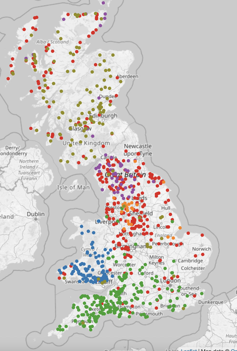
A couple of weeks ago, I released the British Placename Mapper, which is a website that allows you to search place names in Great Britain and show them on a map. You can do searches like finding all the places starting with ‘great’, or ending with ‘burgh’ or containing ‘sea’. I tweeted and tooted about it, and it went a bit viral. Overall, since I launched it on 30th March, it has had over 17,500 visitors who have performed 110,000 searches using it. The average user spent over two minutes on the site, which is quite high for a webpage these days (obviously this is an average, and some people spent ages and others left almost immediately). This post is to share some of the cool things that people have come up with, and the cool places that it has been mentioned online. I’ll do another follow-up sometime in the future to talk about the technical aspects behind the app.
Cool maps
So, first let’s have a look at the cool maps that people created with it. I was very pleased that I managed to make a ‘copy link to these settings’ button on the app, which allowed users to share direct URLs to the specific settings they had configured – this allowed people on social media to share their favourite maps. When listing maps below I’ve tried to include screenshots of the most popular maps (click on them to view them full size), plus direct app links too. These maps aren’t in any particular order, and don’t cover all maps that were made using it – these are just my favourites.
Danelaw area
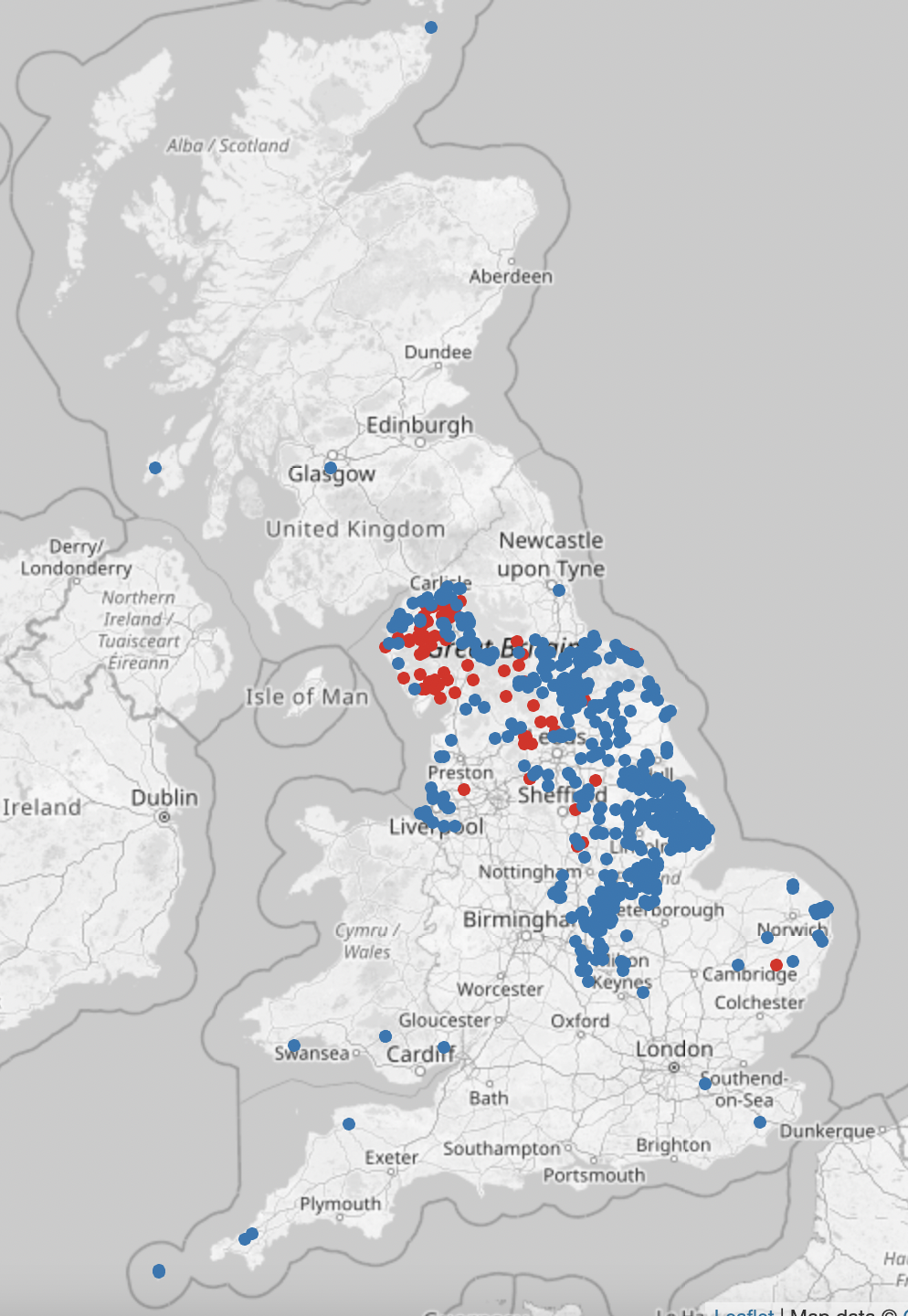
Various people commented that by searching for certain name endings you could pretty accurately show the Danelaw area, defined by Wikipedia as "the part of England in which the laws of the Danes held sway and dominated those of the Anglo-Saxons". This map shows names ending in "thwaite" in red and "by" in blue:
Comparing this to a map of the Danelaw extent (in pink) from Wikipedia shows quite a good match:
Palindromes
This doesn’t tell you anything interesting about history, but it’s still one of my favourite maps here. This map shows places that have palindromic names – that is, they read the same forwards as backwards – like Eye and Notton.
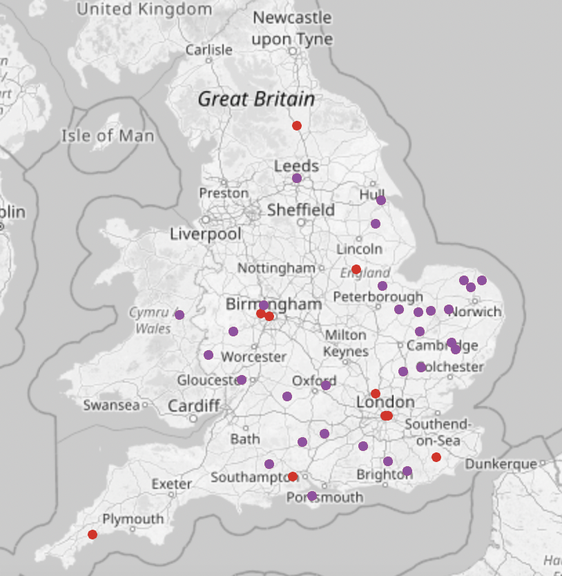
London & Little London
There are a lot more places named after London than I thought there would be, including loads of places called Little London. From a bit more research, the origin of a lot of the Little London placenames are disputed, but there are suggestions they may have come from people escaping the Black Death or the Plague and moving to these villages, or from evacuee’s destinations in the Second World War. See here for the interactive map, and below for Little London in purple, and anything else containing London in red.
Ham/Ley
These two common endings show that they’re nearly all in England, and there are particular concentrations of one or the other – for example, "ham" in East Anglia, and "ley" in the West Midlands, Lancashire and Yorkshire.
Street
Names ending in "street" seem to be concentrated in southern East Anglia and Kent, but do exist elsewhere – see here.
Higher/Upper
This is fascinating: places containing "higher" only seem to occur in Devon/Cornwall and Lancashire, whereas "upper" is spread more evenly throughout a lot of the south and the midlands of England. See here:
Bourne
In British English, a "bourne" is an intermittent stream. I’m sure someone with more geological knowledge than me could link some of the clusters on this map to the underlying geology.
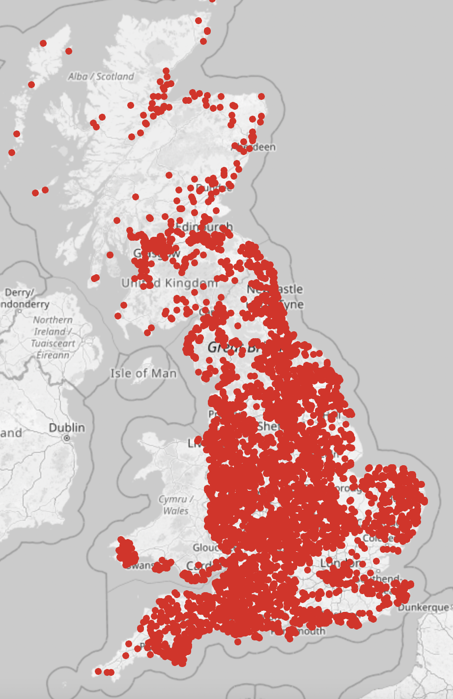
Ton
There are some fascinating patterns with the suffix "ton", in this map. The gap in a ring around London – where there are places ending in "ton" in London and away from London, but not in a ring around parts of the home counties, is interesting – someone on Twitter referred to this as the "Saxon gap", but I can’t find anything about it online. There are also some very distinctive clusters in South Wales – I wondered if these may be related to English-speaking parts of Wales, but a number of the places seem to be in quite rural areas – including relatively remote areas on the West coast. Interesting!
le
Searching for le as a separate word finds places like Thorpe le Street and Chapel-en-le-Frith, which all seem to be concentrated in northern England. It seems strange to have what sounds like a French-inspired part of a name so far away from France, but I’m sure it’s due to some sort of invasion from someone at some point.
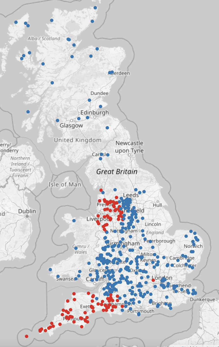
Cornwall
Looking at places starting with tre clearly outlines Cornwall (stopping very sharply at the Tamar) and Wales, and worthy seems popular in Corwall and Devon.
Fosse
Place names with fosse in them clearly outline the path of the Fosse Way a Roman Road:
Church/Kirk
As expected, the church/kirk split is a north/south split, but I was surprised how far south the usage of the word kirk came, with the most southerly examples well into the midlands.
Valleys
This map shows a range of words for "valley", from various languages brought by various peoples. They pretty neatly divide the country into chunks – note the very clustered group of places containing "clough".
Red/Green/Blue
When looking at a map of places including these colours I was expecting to see relatively few places with "blue" in the name (there aren’t that many things in nature that are blue), but was surprised how many places with "red" in the name there were.
Some others:
royd: in Yorkshire, an area of cleared forest land was known as a "royd" and this appears in a tight cluster of place names
names for streams: this shows various different names for a stream (beck, brook etc)
less common letters: there are still quite a lot of places with "z", "q" and "j" in their names
apostrophes : this shows apostrophes anywhere in the name, compared to apostrophes surrounded by letters (like John O’Groats). There are loads of places in southern England named after people (X’s Corner, X’s Green etc).
prime ministers: the surnames of recent-ish British Prime Ministers gives a few potentials for map-based political jokes (if you’re into that sort of thing…)
US placenames – who knew there were so many places in the UK called California?!
One final interesting thing is this tweet and the responses to it. Someone has compared the map of "thwaite" and "kirk" and compared it to a species abundance map for the plant Sand Leek and they match extremely closely. I’ve no idea what this means, and if it is causal – but it’s definitely interesting.
Places it was mentioned
As well as going a bit viral on social media, the placename mapper was mentioned on:
Hacker News – some of the comments are interesting
As well as being mentioned in these places, I got a lot of nice tweets and comments saying how interesting people have found it, which was very pleasing.
I’m hoping to do some extensions to this work in future – maybe for other countries, or for other names in the UK (this only included settlements – but I could extend it to include names of rivers, lakes, forests, mountains etc). Drop me a comment, an email, a tweet or a toot to let me know what you’d like me to do next (and if you really enjoyed this app then please feel free to buy me a coffee).
Summary: You can use QGIS expressions to set the default path for an Attribute Form to be something like @project_folder || '/' || 'MapGraphs', which gives you a default path that is relative to the project folder but also has other custom subfolders in it.
I spent a while redrafting the title of this post to try and explain it well – and I don’t think I succeeded. Hopefully search engines will pick up what I’m talking about from the contents of this post.
So, you may be aware that in QGIS you can set up an Attribute Form which you can configure to pop up when you click on a feature. This can be used to display information about the feature (from its attribute table) in a nice way. See the QGIS docs for more information about this feature.
The bit I’m going to talk about specifically today is display images in these forms. There are various use cases for this, but in my case I had created a static PNG image of a graph for each feature, and I wanted this to be displayed in QGIS when I clicked on the feature. Note that here I’m focusing on displaying data that is already in the attribute table for my layer, rather than editing and adding new features to the layer – because of this, some of the labels for the settings may not sound quite right.
Anyway to set this up for a layer, go to a layer’s properties dialog and choose the Attribute Form tab on the left. You can then switch the mode at the top to ‘Drag and Drop Designer’ and then select the attribute field that has your image filenames in it. You’ll see a wide selection of options, looking a bit like the screenshot below (click to enlarge):
You need to choose a Widget Type of Attachment and a Storage Type of Select Existing file. We’ll come back to the Path selections in a moment. For now, scroll down a bit and choose a Type of Image under Integrated Document Viewer.
That will set up a basic image viewer – but the key part is telling QGIS where the files are located. Look at the dropdown labelled Store path as, in it you have three options:
Absolute Path will expect to see the full absolute path to the image file. For example, on my Mac that could be /Users/robin/GIS/image.png or on a Windows machine that could be C:\Users\Robin\Documents\GIS\image.png. This is probably the easiest way to do this – just make sure that all the filenames in your attribute table are absolute paths – but it is by far the least flexible, and it won’t work if you send the QGIS project to anyone else, as /Users/robin/GIS probably won’t exist on their computer!
Relative to Project Path is a pretty good choice – it allows you to specify relative paths, in this case relative to where your .qgz file is stored. For example, your attribute table could have entries like MapGraphs/image.png and as long as the MapGraphs folder was in the same folder as your QGIS project file then everything would work. However, this means that your attribute table has to have knowledge of what folder your images will be stored in. That’s why I prefer the last option…
Relative to Default Path – this specifies that all of the paths are relative to whatever you’ve entered in the Default path field just above this dropdown. The standard way to do this would be to just select a folder for the Default path field, and all of your image paths will be relative to this folder. For example, if you select /Users/robin/GIS/MapGraphs as your default folder, then your attribute table values can just be image.png and image2.png and it will work.
However, there is a way to combine the best parts of Relative to Project Path and Relative to Default Path by using QGIS expressions. In this case, I wanted to make my QGIS project ‘portable’ – so it could be used on different computers. This meant that everything had to be relevant to the project path somehow (we couldn’t have any absolute paths). However, I didn’t want to store folder paths in my attribute table – I was writing the attribute table contents from a separate Python script and didn’t want to update that every time my folder structure changed. I wanted my attribute table to just contain image.png, image2.png etc (in my case, the filenames were the names of measurement sites for various environmental variables).
So, to give the final answer to this, you can click the button next to the Default path field and choose to enter a QGIS expression. You’ll need an expression like this:
@project_folder || '/' || 'MapGraphs'
This sets the default folder to whatever the current project folder is (that’s the folder that contains the .qgz file), then a / and then another folder called MapGraphs. This is giving you the best of both worlds – a path relative to the project folder, but also being able to specify the rest of the path.
I hope that’s been useful for you. My only question is whether there is any way to repeat fields in a QGIS form. I imagine there isn’t – as the forms are designed for entering data as well as viewing it, and it makes no sense to enter data for the same field twice – but it would be very useful if there was, as then I could have a single attribute called filename (which might contain Southampton.png or Worcester.png) and then have multiple image viewers, one with a default path set up to point to WaterGraphs/ and one to AirQualityGraphs/ etc. I’ve kind of done this at the moment, but I had to duplicate my attributes to have filename1, filename2 etc – which feels a little messy.
In 2019 I wrote about some of my favourite books I read that year and I never got round to doing a follow-up post with books from 2020, 2021 etc. Finally, in 2024 I’m actually going to write up some of these books.
I’ve read around 90 books since the start of 2020, and a lot of these were very good – so I’m going to do this post in a number of parts, so as not to overload you with too many great books at once.
So, part 1 is going to be the first chunk of non-fiction books that I want to recommend. I’ve tried to roughly categorise them, so, let’s get started with the first category:
Space books
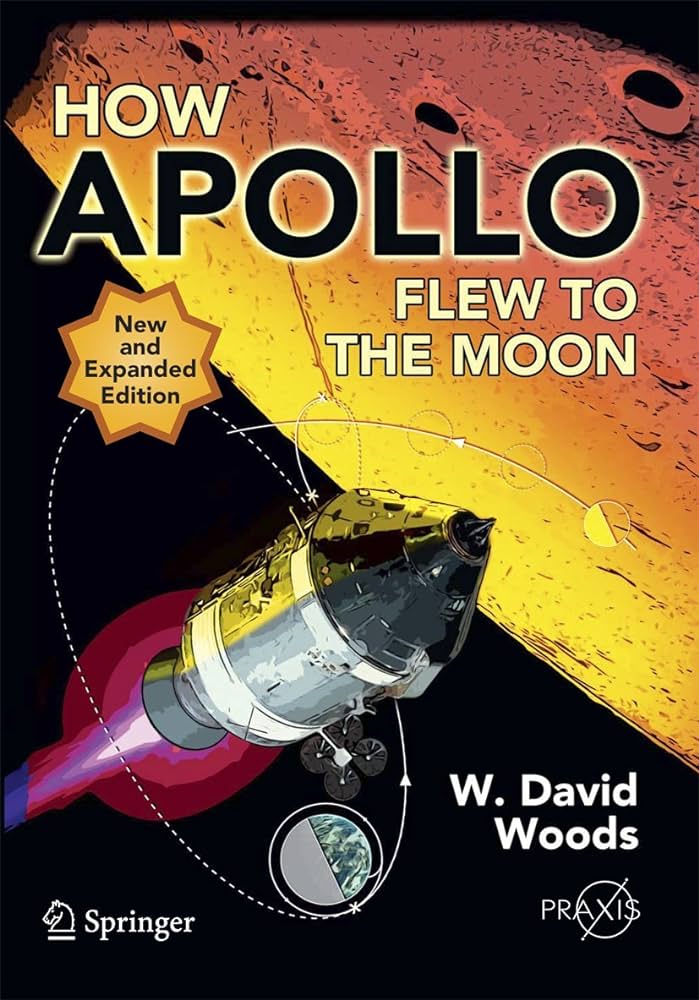
How Apollo Flew To The Moon by W. David Woods
Amazon link
This is an utterly fascinating book. It’s long, and it’s detailed – but that just makes it better (in my opinion). It covers a lot of technical detail about exactly how the Apollo missions and spacecraft worked – to literally answer the question of how they flew to the moon. All phases of flight are covered, from launch to splashdown, with details about each stage of countdown, how details of engine burns were passed to the crew (with worked examples!), how on-orbit rendezvous worked and more. It is liberally sprinkled with images and diagrams, and includes lots of quotes from the Apollo astronauts (from during the missions themselves, as well as from debriefs and trainings). This book is first on the list because it was genuinely one of the best books I’ve read – it was so fascinating and so well-written that I kept smiling broadly while reading it!
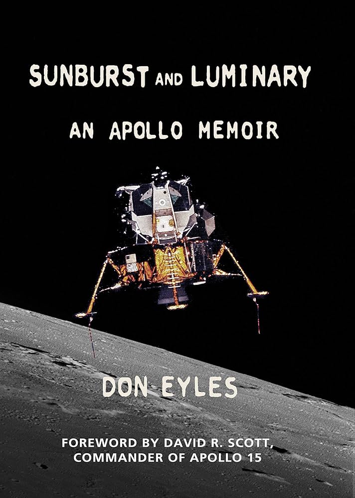
Sunburst and Luminary: An Apollo Memoir by Don Eyles
Amazon link
Another Apollo book now – but this time more concerned with the technicalities of the computing technology used during Apollo. The author was a computer programmer working on code for the lunar module computer, specifically the code used for the lunar landing itself. This book is definitely a memoir rather than pure non-fiction – it covers parts of the author’s life outside of Apollo – but that makes it less dry than some other books on Apollo computing (eg. Digital Apollo, which I never quite got into) but it still covers a lot of technical information. I never fail to be amazed by the complexity of the computing requirements for the Apollo missions, and how they managed to succeed with such limited hardware.
Into the Black by Rowland White
Amazon link
Now we turn our attention to the Space Shuttle. This book covers the first flight of the space shuttle and includes a massive amount of detail that I hadn’t known before. I won’t spoil too many of the surprises – but there was a lot more military involvement than I’d realised, and some significant concerns about the heat shield tiles (and this was decades before the Columbia accident). It’s very well written, with a lot of original research and quotes from the astronauts and original documents. Highly recommended.
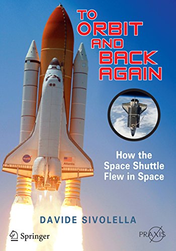
To orbit and back again: how the Space Shuttle flew in space by Davide Sivolella
Amazon link
This is the space shuttle equivalent of How Apollo Flew to the Moon. It is also fascinating, but not quite as well written, and therefore a bit harder to read. I got a bit lost in some of it – particularly the rendezvous parts – but the details on the launch, the computer systems, the environmental systems and tiles were fascinating.
Law books
This might be an unexpected category to find here, but I really enjoy reading books about law – mostly ones designed for lay-people. I’ve read all the typical books by people like the Secret Barrister – these are a few more unusual books.
What about law by Barnard, O’Sullivan and Virgo
Amazon link
This book has the subtitle ‘Studying Law at University’, but you can completely ignore that bit – it is a great book for anyone. With that subtitle you might expect it to cover how to choose a law course or the career progression for a lawyer – but instead, it ‘just’ gives a great introduction to all the major areas of UK law. It is absolutely fascinating. Chapters introduce law in general and the approach lawyers and law students take to the law, and then there are chapters for each major branch of UK law (criminal, tort, public, human rights etc). Each chapter then discusses the various principles of that branch of law and usually goes into detail on a few example cases. I found these examples to be the best bit – thinking about exactly what the law says when compared to the facts of the case, and what bits of law had to be decided by the judge or jury. It gave me a real appreciation for how much the law has to be "made up" (probably a bad choice of words) by the people interpreting it, as an Act of Parliament can never cover everything in enough detail. Note: Try and get the latest edition (3rd Ed at the time of writing) as there are interesting new bits about Brexit, and they cover the Supreme Court rather than the Law Lords.
Court Number One: The Old Bailey Trials that Defined Modern Britain by Thomas Grant
Amazon Link
This book gives a fascinating overview of various key trials that were held in the UK’s most famous courtroom – Court Number One at the Old Bailey. As well as talking about the trials themselves, the author covers the details of the case, and a lot about what life in Britain was like at the time of the trials, to give good context. I was really quite disturbed by the number of fairly obvious miscarriages of justice that were described here – but it was fascinating to hear the details (I’d heard of some of the cases before, but some were completely new to me).
The Seven Ages of Death by Richard Shepherd
Amazon link
This is a fascinating book, but you should be warned that it is quite upsetting at times, particularly in the chapter dealing with the deaths of babies and young children. I actually preferred this to Richard’s previous book (though I enjoyed both) – in this book he talks less about his personal history. Instead, he splits the book up into sections relating to different ages of people at their death. He talks very interestingly about the causes of death he sees at various different ages, and the general changes in people’s bodies that you’ll see at various ages (eg. bones that haven’t yet fused in children, damage due to drinking or smoking in middle age, changes in the bodies of elderly people). As well as discussing the bodies in detail, he also covers details of some of the cases, some of which are quite shocking.
Right, I think that’ll do for Part 1. Next time we’ll look at transport and Cold War books.
I came up with an interesting plan for an artistic map recently (more on that when I’ve finished working on it), and to create it I needed to be able to calculate a large number of driving routes around Southampton, my home city.
Specifically, I needed to be able to get lines showing the driving route from A to B for around 5,000 combinations of A and B. I didn’t want to overload a free hosted routing server, or have to deal with rate limiting – so I decided to look into running some sort of routing service myself, and it was actually significantly easier than I thought it would be.
It so happened that I’d come across a talk recently on a free routing engine called Valhalla. I hadn’t actually watched the talk yet (it is on my ever-expanding list of talks to watch), but it had put the name into my head – so I started investigating Valhalla. It seemed to do what I wanted, so I started working out how to run it locally. Using Docker, it was nice and easy – and to make it even easier for you, here’s a set of instructions.
Download an OpenStreetMap extract for your area of interest. All of your routes will need to be within the area of this extract. I was focusing on Southampton, UK, so I downloaded the Hampshire extract from the England page on GeoFabrik. If you start from the home page you should be able to navigate to any region in the world.
Put the downloaded file (in this case, hampshire-latest.osm.pbf) in a folder called custom_files. You can download multiple files and put them all in this folder and they will all be processed.
Run the following Docker command:
docker run -p 8002:8002 -v $PWD/custom_files:/custom_files ghcr.io/gis-ops/docker-valhalla/valhalla:latest
This will run the valhalla Docker image, exposing port 8002 and mapping the custom_files subdirectory to /custom_files inside the container. Full docs for the Docker image are available here.
You’ll see various bits of output as Valhalla processes the OSM extract, and eventually the output will stop appearing and the API server will start.
Visit http://localhost:8002 and you should see an error – this is totally expected, it is just telling you that you haven’t used one of the valid API endpoints. This shows that the server is running properly.
Start using the API. See the documentation for instructions on what to pass the API.
Once you’ve got the server running, it’s quite easy to call the API from Python and get the resulting route geometries as Shapely LineString objects. These can easily be put into a GeoPandas GeoDataFrame. For example:
import urllib
import requests
from pypolyline.cutil import decode_polyline

# Set up the API request parameters - in this case, from one point
# to another, via car
data = {"locations":[ {"lat":from_lat,"lon":from_lon},{"lat":to_lat,"lon":to_lon}],
        "costing":"auto"}
# Convert to JSON and make the URL
path = f"http://localhost:8002/route?json={urllib.parse.quote(json.dumps(data))}"
# Get the URL
resp = requests.get(path)
# Extract the geometry of the route (ie. the line from start to end point)
# This is in the polyline format that needs decoding
polyline = bytes(resp.json()['trip']['legs'][0]['shape'], 'utf8')

# Decode the polyline
decoded_coords = decode_polyline(polyline, 6)

# Convert to a shapely LineString
geom = shapely.LineString(decoded_coords)
Note that you need to pass a second parameter of 6 into decode_polyline or you’ll get nonsense out (this parameter tells it that it is in polyline6 format, which seems to not be documented particularly well in the Valhalla documentation). Also, I’m sure there is a better way of passing JSON in a URL parameter using requests, but I couldn’t find it – whatever I did I got a JSON parsing error back from the API. The urllib.parse.quote(json.dumps(data)) code was the simplest thing I found that worked.
This code could easily be extended to work with multi-leg routes, to extract other data like the length or duration of the route, and more. The Docker image can also do more, like load public transport information, download OSM files itself and even more – see the docs for more on this.
Check back soon to see how I used this for some cool map-based art.