I have just set up a new home server (a review of which will be coming soon) and have been installing various programs that I want to run on it. A number of these are servers, such as sshd, apache, samba etc. All of these have fairly easy installs under Debian and will automatically run at startup, and can be controlled by /etc/init.d scripts.
However, I also have a number of other programs I want to run as services, constantly in the background, which don’t come with nice Debian init.d scripts. After asking a question on SuperUser I found that one fairly simple solution would be to use a set of tools called daemontools. These tools provide a simple way of defining services which run constantly, and can be controlled by an administrator (in a similar way to /etc/init.d services). daemontools seem to be designed very well, and are quite easy to use, but the documentation on the website seems to lack a simple quickstart guide…so I thought I’d write my own.
At this point I should mention that I have only been using daemontools for a few hours, so I could be completely wrong about anything I say below. These instructions will be for Debian, but should be fairly easily to use with other distros (the only bit that will be significantly different is exactly how to install it with the package manager). Anyway, proceed at your own risk!
Install daemontools
In debian you will need to run apt-get install daemontools daemontools-run (both packages are important – I didn’t install the latter package and it caused me lots of frustration). This will install the tools themselves and also add the required lines to startup files to ensure that all of the required daemontools services start when the machine boots.
Create a service directory
You will probably find that the installer has created a /service directory for you. If it hasn’t then create one yourself. Then create a directory under that directory for each service that you want to run. Here we will be creating a test service, so create a directory called test. Run chmod 1755 on this directory.
Create the service run file
daemontools needs to know what command(s) you need to run for this service, and these commands should be put inside a shell script called run in the service directory. For example, the file could contain:
#!/bin/sh
echo Running service
exec some-command-here
Finished!
That should be all you need to get the service running. You should probably restart the machine now as that will ensure that all of the daemontools monitoring services have started correctly. Once the machine has started the new service should have started running. If it crashes or ends for some reason it will restart after one second. Any new services you add (which you can do exactly as above) should start within five seconds. You can use the svc command to control the services you have created (see man svc for details)
Summary: Very useful for reference while producing graphs, and very comprehensive (including heat-maps, 3D graphs and maps).
Reference: Mittal, H. V., 2011, R Graph Cookbook, Packt Publishing, Birmingham, UK, 272 pages, Publisher’s Website
As a scientist I often need to plot graphs of my data, so I am keen to learn more about how to do this in various languages. I tend to use R for most of my statistical analysis, so plotting graphs in R is something that I often need to do. I have a bit of knowledge about R already (mainly gained from the books that I have previous reviewed about R), and looked to this book to explain more about graphing in R. As stated in the title it is a ‘cookbook’ – a type of technical book that provides a number of ‘recipes’ for performing various tasks, and this is both one of the main advantages and main disadvantages of this book.
I generally have a love-hate relationship with these ‘cookbook’-style books – I find them useful when wanting a quick answer to something, but I am slightly concerned about the manner in which the teaching/learning takes place. These books can be very useful, as the cookbook style allows the reader to very quickly learn how to do something which they need to do, but this learning does not always take place within a context which allows the reader to understand why they are doing what they are doing. For example, in a book like this, the reader could be told exactly what commands to type to plot a line graph – but they may not actually learn anything about what each of these commands do, and how to adjust them if they need to do something very slightly different.
However, I am pleased to say that this book is actually very good. It starts with an overview chapter that contains basic recipes for plotting various types of graphs (all of which are covered in greater detail later on in the book) as well as exporting the graphs to be used in other documents. Then comes one of the most important chapters – a detailed explanation of the par() command for adjusting parameters such as margins, colours, fonts and styles. Again, this is presented in ‘recipe’ form (of which more below) which again is a double-edged sword: it makes it easy to find the parameter setting you’re looking for, but harder to get an overview of the range of different parameters you can set. A simple table at the end of this chapter listing the parameters and the possible options for each of them would have been very useful – but was sadly not included.
The rest of the book goes through a number of types of graph, providing detailed recipes for creating them. They start with the most important types of plot: scatter graphs and line graphs (with a helpful emphasis on plotting time-series data with sensible axes labels) before moving on to bar charts, pie charts, histograms and box and whisker plots. All of this would be expected in a book on graphing software – however, this book goes further by providing a section on heat-maps and contour plots, and then a section on creating maps. The heat-maps section is particularly interesting, and I can see a number of applications of the example visualisations they have provided. The book then closes with a chapter on exporting graphs for display – both to raster and vector formats.
As mentioned already, all of the information is provided in the form of ‘recipes’, which have a standard format of: introduction, getting ready, how to do it, how it works…, there’s more… and see also. This tends to work well for most parts of the book – with the introduction explaining the type of graph and why you might want to use it, getting ready showing you how to load the required libraries, how to do it providing code and how it works explaining the code, with more options being explained in there’s more and see also. However, this falls down slightly when dealing with topics that require a little more explanation – such as the section on exporting graphics for publication, which could really do with having a more detailed section on the difference between raster and vector output, and how to choose between them.
The book generally choses sensible datasets to plot for each graph, although at times the code is made unnecessarily confusing by adding lots of code to download datasets via web APIs (useful to be able to do, but perhaps not hugely relevant to the topic of this book). Apart from this, the code is generally well written, although some extra comments in the code might have been helpful – as it would save me constantly referencing between the how to do it and how it works sections.
Overall, I will definitely keep this book on my shelf as a handy reference for when I need to create a graph quickly in R, although I would recommend combining this book with another book (for example R in a Nutshell) for more details on the graphing functions and the rest of R.
(Disclaimer: I was given a free review copy of this book)
I’ve recently moved in to a new flat, and have bought lots of bookcases to store all of my books. Of course, I had the terrible decision to make of how to arrange all of my science books. I mean I could categorise them fairly easily (maths, physics, biology etc), but what order do I put these in?
When thinking of this I thought of the xkcd comic below, and had an idea:
Why not arrange them by ‘purity’? Well – that’s what I did (see below):
I should point out that computing is definitely not purer than mathematics, but it is on the top shelf as that is the only shelf that my fiancee can’t reach, and she rarely (if ever) uses those books. Apart from that though, it is pretty much in purity order…
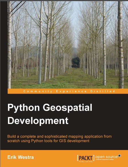
Summary: Great book – both for GIS concepts and for teaching Python libraries. Lives up to the boast on the front cover – you really will learn to create complete mapping applications, learning a lot of useful tools and techniques on the way.
Before I start this review I should probably point out that I am a PhD student working in Remote Sensing and Geographical Information Systems, so I expected to know a fair amount of the theory in this book. The reason I wanted to read it though, was to learn how to do this analysis using Python and its associated libraries. This book succeeded in teaching me how to use Python to perform geospatial analyses, and actually taught me a significant amount of wider GIS knowledge which I had not picked up through any of my university courses.
The book is divided into four main sections: the first introduces general GIS concepts, the second explains basic GIS operations in Python, the third shows how to use databases with geographic data and the fourth combines all of the previous information into two GIS web-apps. It is always difficult to work out what level to pitch this sort of book at – as a number of potential readers will already have experience with GIS (and are using the book to learn about doing GIS analysis in Python, like me), but some will be complete beginners who want to introduce map-based analysis into their applications. The first few chapters of this book are pitched nicely at a mid-point between these two reader groups: the author explains things clearly and precisely without seeming patronising. Although I already knew much of the basics, I found the section on projections and co-ordinate systems very useful as I had never properly understood these (I’d always seen the different options in software I was using for Projected Co-ordinate Systems and Geographic Co-ordinate Systems, but I never knew the difference until I read this book!).
The next section explains how to use a number of Python GIS libraries such as GDAL/OGR, PyProj, and Shapely. The author starts with a general description of the capabilities of each library, and continues with a ‘cookbook-style’ approach showing how to do various tasks with these libraries. For example, instructions are given for how to convert projections and calculate Great Circle Distances with PyProj, how to extract shape geometries and attributes from shapefiles using OGR and how to do basic GIS analysis with Shapely. Details are given on joining these libraries together to exchange data between them using the very useful Well-Known Text (WKT) format – a format that I hadn’t come across, but which appears to be very useful. This section finishes by putting together a number of these libraries to do some real-world tasks such as identifying parks near urban areas.
The third section focuses on geodatabases – an area I know very little about. This section gives a good overview of the concept of a geodatabase, and then specific details about three geodatabases: PostGIS, MySQL and SpatiaLite. I was pleased to see that three contrasting databases were chosen, and a good listing of advantages and disadvantages of each was given. After introducing the workings of these databases, code examples for linking them to Python are given, starting from basic queries and going right up to complex spatial analysis performed within the database. A geospatial application (called DISTAL) is then implemented, showing how to combine geodatabase access with the GIS analyses explained in the previous section. This is implemented as a web-application, but previous experience with web programming is not needed as it is implemented using simple Python CGI scripts, and there are sidebars explaining terms that the reader may not have come across before.
The fourth section is by far the most complicated, and deals with producing maps using a library called Mapnik and producing geo-enabled web-applications using GeoDjango. I must admit that I didn’t quite follow all of this chapter, although this is probably because I’m not hugely interested in, or experience with, building web-apps. In some ways a little too much emphasis is made of how to do things using Django – and trying to introduce any web-app framework (be it Django, Ruby on Rails, or anything else) in one chapter is a tall order – and not enough on the GIS, but I can see why the author included it – as it brings together a fair amount of the tools covered in the book into one coherent whole.
Overall, I’m very impressed with this book. If I had my way (and you never know, if I end up as a lecturer one day I might…), I’d make Chapter 2 part of the core reading for any GIS course, as I am completely shocked that it covers areas that I have never covered even when doing Advanced GIS courses at degree level! I should mention that as well as the chapters mentioned above there is a useful chapter on sources of geospatial data (which, again, mentioned sources that I’d not heard of), and a comprehensive index which makes it very easy to find things. The instructions on how to use the Python libraries (and, more importantly, how to join them together) are well-written and comprehensive and the introductions to GIS concepts are pitched at just the right level. I would thoroughly recommend this book for any GIS or geospatial data user for two main reasons: firstly, it gives great introductions to GIS concepts they may not have come across, and secondly, knowing how to do these things in Python can make certain jobs so much easier (how about a 10 line Python script rather than a few hours of repetitive data conversion?).
(Disclaimer: I was provided with a free review copy of this book)
I spent part of today struggling with an undergraduate student to get our university-provided ArcGIS dongle licenses to work. In the spirit of sharing our hard work with the rest of the world, the solution below may be of use to people. The error that we got which were fixed by this solution are listed below, but it may be worth checking this solution anyway, as the licensing errors given by ArcGIS don’t always seem to have much relation to the actual problem.
FLEXnet Licensing error:-96,7 System Error: 11004 "WinSock: Valid name, but no record (NO_ADDRESS)"
We also found that the ArcGIS License Manager service would not start correctly – it would attempt to start and then stop immediately. When getting this error I originally thought that it meant that the name of the license server (that is, the name of the local machine) was not properly set in the ArcGIS Desktop Administrator application, but it turned out that it was set correctly there. After much Googling and trial and error I found that the license file looked a bit like this:
--------------
START_LICENSE
SERVER xxx ESRI_SENTINEL_KEY=37135503 27004
VENDOR ARCGIS
FEATURE ARC/INFO Â Â Â ARCGIS 9.0 30-aug-2011
......
In the extract above you can see the SERVER xxx bit. I turns out that the xxx needs to be replaced with the name of the server. This is normally done by systems administrators for networked license servers, but if you are using a dongle you may need to do it yourself. Simple change SERVER xxx to SERVER TheNameOfYourComputer, and the license manager service should start properly and you should be able to run ArcGIS.
Please let me know (by the comments below) if this works for you. Beware that it is unlikely to work for ArcGIS 10.0, as I believe the licensing model has changed.
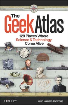
Summary: Very interesting, and great fun for a geek like me! Now I just need to find the time/money to visit these places…
Reference: Graham-Cumming, J., 2009, The Geek Atlas, O’Reilly, 544 pages O’Reilly Link
I’m a great fan of John Graham Cumming’s blog, so when the chance came to review his book, The Geek Atlas, I jumped at it. The book is part travel guide, part popular science textbook. It provides information about 128 ‘geeky’ places to visit around the world and provides brief introductions to the science behind the places mentioned. After reading the Table of Contents I realised that this was definitely a book for me: I’ve been to 12 out of the 128 places mentioned already, and would love to visit most of the others. In fact, I spent the next hour going through them with my fiancee and trying to work out when we’d be able to visit some more of them…
Anyway, back to the review. The places listed in the book are all interesting for some reason or other: they range from museums, churches and graveyards to company training centres and ex-military bases. The ‘interestingness’ is normally provided through some link to science or technology, an area that most people who self-identify as ‘geeks’ find very interesting. However, the author seems to have gone to great lengths to make this more than just a simple list of places to visit, and has provided very readable introductions to the science and technology behind the places. These brief introductions cover topics such as suspension bridges, natural selection and breaking the Enigma code. At times it feels that they assume a little too much of the reader (sometimes there are some rather scary looking equations which I suspect many readers would not understand), but they are generally pitched at an appropriate level. The description of Bayes Theorem, for example, is by far the best I have ever read (significantly better than the descriptions in a number of probability and statistics textbooks I have read).
As for the geographical distribution of the places, the majority are in Europe and America, with the highest concentrations in the UK and USA. Although I could easily predict some of the places on the list (for example, I knew that the Science Museum would be on the list, as would Bletchley Park), there are a number of more unusual places like the British Airways Flight Training Centre (where you can use the same flight simulators that real pilots use) and the Cherynobl Exclusion Zone (which apparently is fairly safe to enter these days). It is impressive how much science is covered in the book – from 17th century work by Newton right through to the design of the new Airbus A380 aircraft – and this is shown by the number of cross-references in the book. One of the attractions is a cemetery where a number of famous scientists were buried, and nearly all of these scientists had been covered, at least to an extent, elsewhere in the book.
I can’t really think of much more to say, other than to note that the book is quite thick and has enough interesting places in it to keep you going for a number of years. On that note – I’m off to plan some travelling…
(Disclaimer: I was provided with a free review copy of this book)
I’ve spent the last couple of months getting used to my new MacBook Pro, and I must say that overall I’m really liking it. Continuing my previous posts about my mac, here are my favourite three pieces of OS X software:
Preview
This is the built-in image and PDF viewer that comes with OS X. Not very exciting, you might think, but it is actually a very powerful piece of software. As well as viewing images and PDFs (including lovely smooth scrolling and zooming) it will let you modify them in a variety of useful ways. For example, you can re-order pages in PDFs, combine two (or more) PDFs into one file, and crop PDFs and images. You can also annotate files with highlighting, texting, freehand drawings and any other type of annotation you could think of. Finally, the search feature in PDFs is the best that I’ve ever seen in a PDF reader. Yes, I sound slightly too enthusiastic about this, but I’ve never before found a free, easy-to-use piece of software that has this power when viewing and editing PDF files.
(I can’t provide a download link as it is built-in to OS X)
NetNewsWire
This is a free (ad-supported – you can pay to remove the ads) RSS feed reader for OS X. It’s fast, easy-to-use, and, most importantly, can be controlled entirely with the keyboard. It also displays pretty much everything that is in the original blog post, so if there is a YouTube video inside a blog post then you can play it from within NetNewsWire. This is one of the apps on my list to buy a license for when I have some money…
This is an unusual app, but it is incredibly useful for those of us who move around a lot with their laptops. For example, as a PhD student I spend time at home, my office at the university, other work rooms at the university (labs and so on) and various other places. Airport Location will work out where you are based on various pieces of information (such as the wireless network you’re connected to, your IP address or your geolocation information) and then change loads of OS X and application settings to make them appropriate for that location. The upshot of this is that when I get to my office my laptop is automatically muted, Skype is set to away, and my default printer is set to the local networked printer, and the opposite happens when I get home.
Git is my favourite version control system (see Why is Git better than X for some good comparisons with other tools, and my GitHub repositories to see what I’ve been doing with it lately). I now use it for all of my programming projects, and many of my writing projects (as I’m now using LaTeX for nearly all of these).
DTerm is a simple utility for OS X which provides a drop-down Terminal in the Finder. The best way to explain it is with a screenshot (see below). When in any Finder window, press Cmd-Shift-Enter, and the DTerm dialog will pop up. You can type any terminal command in the box, and it will run it in that folder, or you can press Apple-Enter to open a full terminal at this folder and run the command.
The combination of the two gives what is, for me, the best way to do source control in OSX. I simply use DTerm for all (or most of) my git needs. When I realise I need to get some code into source control, a simple git init in DTerm starts a repository, ready for me to do whatever I want with, and then I just commit using git commit -am "Blah" in DTerm. Simple, fast and all the power of the command-line.
(I must state that I do use GitX (a Git GUI for OS X) sometimes, particularly for viewing commit logs and branch diagrams)
Summary: Very comprehensive and very useful, but not good for a beginner. Great book though – definitely has a place on my bookshelf.
Reference: Adler, J., 2010, R in a Nutshell, O’Reilly, Sebastopol, CA, 611 pagesO’Reilly Link
After reviewing a book about R designed for beginners (see my previous post) I thought I’d step up the pace slightly and look at a more advanced book. I’m pleased to say that I was not disappointed. This book is so comprehensive – you can find nearly anything you want in it!
The book starts with a brief, but comprehensive, R tutorial. This tutorial is rather light on actual statistics, but gives a very good introduction to the syntax of the R language. This focus on the language continues through the whole of Part II, which contains detailed chapters on the language, syntax, objects, symbols, functions and high-performance programming in R. This is very different to most books on R which jump straight into the statistics. Although this part may seem rather boring to some, it provides a very good grounding in the basics of R programming, which make the rest of the book significantly easier to understand.
Through reading Part II I learnt a huge amount about the R language – finding out some things that I never knew, and realising how many things that I did know actually worked. This part may well confuse those with no previous programming experience (see my comments on this later), but those who are at least slightly familiar with the terminology, it gives a very comprehensive explanation of the language itself.
Part III is where the book starts to get into R’s main use: statistics and statistical graphics. Very sensibly, this section starts at the beginning of the process with how to import data (including instruction on how to connect R to databases) and then a lengthy (over thirty pages) section on preparing data for analysis. This is incredibly useful as this can often take a significant proportion of the time spent on a project. The graphics chapters after this provide a comprehensive introduction to the standard (‘base’) graphics system, and then the lattice graphics system. I’m glad to see that a non-base-graphics system is given space in this book. From what I’ve seen on the web, it seems that very few R programmers use the base graphics system for producing production graphics, so this is a sensible inclusion.
Finally, after all the preparation, we get to the statistical analysis section (Part IV). Of course, as the book has covered so much of the fundamentals earlier, the statistics section can fly along, focussing mainly on the statistics themselves and the syntax of the tools that R provides, rather than the mechanics of how to write valid R commands. A wide range of statistical tests are included, and they are covered in a very sensible order (in fact, almost exactly the same order that my statistics class covered them: starting with summary statistics, then probability distributions, on to statistical models and then beyond that to classification and machine learning). I won’t lie and say that I’ve read every word of this section, but the bits I have read have been very good: concise but comprehensive.
There’s not really much more I can say about this book: it has become my ‘go-to’ reference for anything I need to do in R. It would be intimidating for a beginner, but it is not aimed at beginners, so that’s fine. For those of us who are slightly more experienced with R, it is a great book, and I thoroughly recommend it.
(Disclaimer: I was provided with a free review copy of this book)
My fiancee is studying in Lille, France at the moment, and I spent last week with her in Lille, including a two-day trip to Paris. During my time I noticed a number of interesting (or at least semi-interesting) things about life in France:
Pedestrian crossings are scary! When the green man is shown it does not necessarily mean that it is safe to cross. What it actually means is that you are protected from traffic coming straight ahead, but not from those turning right or left. In practice this means that most foreigners (and a lot of natives) sprint across the pedestrian crossings to try not to get killed!
The number of bakeries per capita in France is awesome. Within 30 seconds walk from our hostel there were three awesome bakeries. This pleases me very much.
For some reason nearly every street corner in Paris seems to have a condom machine on it. I have no idea why they need that many machines.
The street sellers at the bottom of the funicular railway in Montmartre are very pushy. Both times we walked past there one of them tried to tie some sort of piece of string to my fiancee’s hand. Strange.
The Paris metro has a lot of lines – 15 standard metro lines, plus 5 RER (a sort of express metro) lines. In comparison London Underground has just 11. This means that they’ve run out of colours for the metro map – meaning that you have a number of lines which are similar colours (particularly greeny-olive-brown colours), making it very difficult to tell the difference (particularly in low-light conditions).
However, the amazing thing about the RER lines is that they have double-decker underground trains (see the picture below). This is awesome.
The Arc de Triomphe is more interesting than I thought – there is a good exhibition in it about historical events that have happened there. The tomb of the unknown soldier is there, and the flame over it is lit every evening.
French railways seem to be a mixture of very high-tech and very low-tech. For example, TGV trains are very fast, and work very well, but their departure boards at Paris Gare du Nord are the old-style clicky boards (the ones that click round loads of times to show the right destination and time).
It’s amazing how much random French I know. For example, the emergency stop signs on all the metro trains have a notice by them saying “… … sera puni”. From the old song Que sera, sera I know that “sera” means “will be”, and therefore not to press the button as I might be punished! Also, trains in France are retarded (actually “retarde”) when they are late, another thing I realised I knew.





 and
 are very good books, and yes I did steal the title idea from him)