So, hot on the heels of my last post, I’m now applying another concept from a computing blog post to science. For many years I’ve been a fan of Joel Spolsky’s blog, and I’ve learnt a lot from it. One of his most interesting posts was called The Law of Leaky Abstractions. As with my last post, I’ll briefly explain the computing context, and then broaden out to talk about its applications to science.
Joel states that the law of leaky abstractions is that:
All non-trivial abstractions, to some degree, are leaky.
Of course, that doesn’t make much sense without understanding what abstractions are, and what it means to say that they are leaky. Joel defines an abstraction as a simplification of something which hides the complex details that are occurring under the covers. Protocols such as TCP/IP are a good example of an abstraction in computing. They abstract the details of  communicating over a computer network., allowing you to send messages across wires and guarantee that they will get there, without having to worry about how it actually works. The problem is that sometimes these abstractions leak – that is, some of the hidden complexity bubbles up to the surface. In the TCP/IP example above this might happen because the network cable has physically broken, or because some of the pins have become crossed, or because of faulty network infrastructure elsewhere.
An example from everyday life is how a home heating system abstracts away the details of actually heating your house, and simply replaces it with a dial allowing you to control the temperature. That all works fine until your radiators get air trapped in them (as happens in my Southampton house worryingly frequently), or the heating pump fails, or the water tank overflows.
Now, these kind of abstractions can be seen in science too. Newtonian mechanics is an abstraction of the underlying complexity of motion which works fine most of the time – until you get to speeds near to the speed of light, at which point it stops working. Another example is atomic theory, which states that all matter is composed of individual atoms. In many situations, this theory works very well, but sometimes the underlying complexity of sub-atomic particles (such a neutrons, quarks or gluons) bubbles to the surface.
Abstractions in all fields often come in sets, or pyramids. For example, the abstraction of writing
print "Hello, world!"
to display some text on the screen has a whole pyramid of abstractions below it, a few examples of which are:
The abstraction that strings can be stored as integers (you only have to look at the difficulty in supporting foreign characters in many programming languages to realise that this abstraction is very leaky)
The abstraction that programs have an unlimited memory address space to use (performance issues caused by page-faults, and error messages about Windows virtual memory show how this leaks)
The abstraction of a filesystem containing files and folders (replacing the complexity of tiny magnetic areas on a hard disk)
This type of pyramid is so common that there is even an official standard for it within the field of computer networking: the Open Systems Interconnection model. This has 7 layers, using abstractions from the simple (transmitting one bit over an electrical link) to the complex (sessions and application protocols).
Similarly, there is a pyramid of abstractions in many areas of science. For example, if you abstract away the behaviour of individual electrons you can produce ‘laws’ of electrical circuits. Combining these laws produces the abstractions of electronics (involving complex circuits and logic gates), and these can then be abstracted away again with the creation of integrated circuits, and so on, until a complex electronic device is created. However, every so often the complexity will bubble up again. For example, the fundamental limitation on the speed of modern computer processors is the size of an electron (as the circuits can’t get any smaller than that) – which is a big leak from the bottom abstraction (electron abstracted into the laws of electrical circuits) to the top abstraction (computer processors which run high-level code).
Now, this all raises some interesting questions – some of which I’m hoping to address in future posts:
Are these pyramids of abstractions present in all areas of science? If not, then why not? I have a suspicion that mathematics will prove to be different…
Is the process of creating these abstractions part of what defines a field as a science? How does the gradual building of the abstraction pyramid link to theories about the progression of science (such as Kuhn’s paradigms)
How does the pyramid of abstractions look in a particular field (for example, my field of remote sensing)? Does thinking about the pyramid of abstractions for your field lead to good ideas for research?
Does ‘good’ (whatever that may mean) research seek to build abstractions, or to demolish abstractions?
Hopefully I’ll get the chance to revisit some of these issues in future posts – but in the meantime please leave your comments.
I listened to a very interesting episode of The Pod Delusion podcast today. In fact, all of the bits of the programme were interesting: from a discussion of faith schools from an athiest perspective, to a description of Tesco’s planning policies from a local council planning officer. However, the item on the programme that I want to talk about was called Default Deny and was written by Sean Ellis. Below I’ll give a brief description of his argument before talking about how I think this applies to academic life.
Sean took his inspiration from an article called The Six Dumbest Ideas in Computer Security, by Marcus Ranum which states that the dumbest idea is Default Accept. Until recently, many computer security systems were designed around the idea of letting everything go through apart from things that were specifically told to be stopped (thus the name: Default Accept). This is easily seen in Windows anti-virus software. Windows (at least before Windows XP) used the Default Accept principle, so anti-virus software was created with huge lists of pieces of software which must be denied. In his article, Marcus Ranum argues that it is far more sensible to base the system on a Default Deny principle, thus only allowing specific software to run.
So far, so good – but what does this have to do with academia? Well, Sean applies this to ideas by asking whether people have Default Deny brains or Default Accept brains, that is: whether they accept any new ideas by default, or whether they immediately reject them until they have studied the evidence and been convinced. He comes to the conclusion that many people have Default Accept brains, but that Default Deny brains would probably be a more healthy situation.
That struck a chord with me, in terms of scientific studies and academia in general. It can easily be said that science must be done with a Default Deny brain (or at least with a Default Deny hat on), but I think there is more to it than this. As a student in secondary school we were expected to work within a Default Accept paradigm. We weren’t expected to question what we were being taught – we were meant to just accept it at face value. That started to change at A-level when we were first introduced to some of the controversy in our subjects. I distinctly remember one of my A-level geography lessons when we were told that scientists still weren’t sure about how drumlins (a type of glacial landform) were formed. I suppose that was the day that I first became really interested in research: I’d found that we didn’t know everything, and I wanted to be one of the people that started to find things out!
However, even though we had been introduced to controversy at A-level we weren’t expected to really question the fundamentals we were taught. When writing an exam essay about the Burgess model I was expected to list a selection of its flaws, but not to question it at a fundamental level, nor to talk about the inherent problems with models.
At the beginning of my undergraduate degree I started to read journal papers: the original places where new scientific ideas are circulated. But, as a new student, I was far too in awe of the authors to criticise their work. After all, how could I, a lowly first year student, find problems in the work of professors and lecturers – especially work which had been accepted by equally experienced peer-reviewers? Gradually, however, I began to realise that it didn’t actually take a huge amount of knowledge to be able to intelligently critique someone’s work. Ignoring the name and affiliation of the author often helped with this. I distinctly remember finding a paper about the Empirical Line Method in a relatively unknown journal (something like the Chinese Journal of Soil Science – a strange place for a remote sensing paper), reading it, and realising that I could have written something better in my sleep! After that they followed thick and fast: I realise that papers in Remote Sensing of Environment are not without their flaws, and my unquestioned acceptance of the Ruddiman hypothesis completely ignored the body of work that presented alternative theories.
The gradual change from a Default Accept paradigm to Default Deny is an important change which occurs during education. Sadly, this doesn’t seem to occur for many people (even students who go on to get good degrees at university), and it should really start far lower down in school (there is no reason why able students should not be questioning the accepted point of view at GCSE level). Science is entirely based around the questioning of facts, and the denying of knowledge that cannot be backed up with evidence. All of my favourite academic papers (and, indeed, most of the important papers ever written in science) came about from the author denying what he has read and heard, and considering alternative points of view. When the change from Default Accept to Default Deny takes place it marks the start of the transition of that individual to a true scientist – and is a mark of increasing academic maturity.
I’ve just gone through a bit of a ‘journey of discovery’ in R while trying to plot a grid of plots for one of the research projects I’m doing. I wanted to write a simple function which could produce this grid of plots from a CSV file, allowing me to easily view the trends of the dune metrics produced by my DunesGIS project.
I first started by loading the data into R and producing a simple ggplot2 graph, which I then customised using the standard ggplot2 commands. At this point I had the following code:
# Load the ggplot2 library
library(ggplot2)

# Read in the CSV file taking into account the headers
df = read.csv("D:\\results.csv", header=T)

# Plot a simple graph
qplot(t, mean_len, data=df, geom="line", xlab="Time", ylab="Mean Length", main="Mean Length")
I wanted to produce a number of these plots to show all of the key dune metrics, so I attempted to arrange these plots in to a grid. This is where it got difficult…
I could easily put the plots in a grid using the arrange function (available here), but I had to write lots of repetitive code to create the graphs. I couldn’t see a way to easily put this into a function, as I needed to take in a variable name as an argument and then use it as a variable. Luckily, some of Steve Yegge’s posts on lisp must have stuck in my brain, as I realised I could do this using a macro.
It happens that R is a nice language that has support for macros, and I managed to write one quite easily:
This uses the defmacro function, and takes a variable name (for example, mean_len) and some text to use as the title, and then returns the result of the qplot() call. Combining this with the call to arrange led to the code below:
# Define the macro (we're adding more options to the plot this time, but it's the same idea)
cg <- defmacro(varname, vartext, expr={qplot(t, varname, data=df, geom="line", main=vartext, xlab="Time", ylab="") +
	scale_x_continuous(breaks=NA) +
	theme_bw() +
	opts(axis.title.x = theme_text(size = 10, vjust = 2, hjust = 0.6)) +
	opts(plot.title = theme_text(size=10, face="bold", hjust=0.7)) +
	annotate("segment", x=-Inf,xend=Inf,y=-Inf,yend=-Inf,arrow=arrow())})

df = read.csv("D:\\results.csv", header=T)

# Create all of the graphs we want, storing them in variables
p_mean_len = cg(df$mean_len, "Mean Length")
p_total_len = cg(df$total_len, "Total Length")
p_max_len = cg(df$max_len, "Max Length")
p_min_len = cg(df$min_len, "Min Length")
p_std_len = cg(df$stdev_len, "StDev Length")
p_mean_cl = cg(df$mean_closeness, "Mean Closeness")
p_std_cl = cg(df$std_closeness, "StDev Closeness")
p_def_dens = cg(df$defect_dens, "Defect Density")
p_r_score = cg(df$r_score, "NN R-score")

# Arrange the plots into a grid
arrange(p_mean_len, p_total_len, p_max_len, p_min_len, p_std_len, p_mean_cl, p_std_cl, p_def_dens, p_r_score, ncol=3)
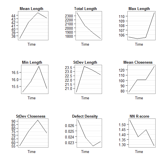
Now, I thought I'd been pretty clever by now, and was pleased with the result (see below). However, I realised it could do with improving...
Grid of plots (arrange-based method)
The graphs weren't aligned very well, and the whole thing looked rather amateurish - not what I want if I end up publishing in a journal. So, I contacted the ggplot2 mailing list for help. You can read the whole thread here if you want, but I'll be explaining how I progressed below.
Members of the mailing list suggested that I used the faceting feature to make a better grid of plots. I had considered this, as I knew faceting created grids of plots, but I'd never really understood this whole facet thing. Still after some help from the mailing list I found I could easily create a 'dummy faceting variable' to get this to work.
Originally, my data frame looked like this:
name
t
n
mean_len
total_len
max_len
min_len
stdev_len
mean_closeness
std_closeness
defect_dens
r_score
z_score
p_value
1
S5_Pe06_sand02
1
64
37
2378
106
15
21
77
55
0.027
1.5
8.3
0e+00
2
S5_Pe06_sand03
2
49
42
2060
105
16
24
101
76
0.024
1.4
5.0
1e-06
3
S5_Pe06_sand04
3
42
45
1881
105
17
23
101
92
0.022
1.4
5.5
0e+00
4
S5_Pe06_sand05
4
40
43
1727
111
15
23
127
73
0.023
1.3
3.4
6e-04
To use faceting I needed to reshape this data frame so that I had a variable field giving the name of the variable, repeated as many times as needed to get all of the data in. That sounds complicated, but comparing the example below to the example above should explain it:
name
t
variable
value
1
S5_Pe06_sand02
1
n
6.4e+01
2
S5_Pe06_sand03
2
n
4.9e+01
3
S5_Pe06_sand04
3
n
4.2e+01
4
S5_Pe06_sand05
4
n
4.0e+01
5
S5_Pe06_sand02
1
mean_len
3.7e+01
6
S5_Pe06_sand03
2
mean_len
4.2e+01
7
S5_Pe06_sand04
3
mean_len
4.5e+01
8
S5_Pe06_sand05
4
mean_len
4.3e+01
9
S5_Pe06_sand02
1
total_len
2.4e+03
10
S5_Pe06_sand03
2
total_len
2.1e+03
11
S5_Pe06_sand04
3
total_len
1.9e+03
12
S5_Pe06_sand05
4
total_len
1.7e+03
13
S5_Pe06_sand02
1
max_len
1.1e+02
14
S5_Pe06_sand03
2
max_len
1.1e+02
15
S5_Pe06_sand04
3
max_len
1.1e+02
16
S5_Pe06_sand05
4
max_len
1.1e+02
This can be easily accomplished using the melt command in the reshape package. The command I used was:
m <- melt(df, id = c('name', 't'))
This performs a melt operation on the data frame df using name and t as ID variables (that is, variables that identify each row - in this case the time and the name of the model run). Once you've melted the data frame you can plot it using the faceting feature of ggplot2, for example, in the code below:
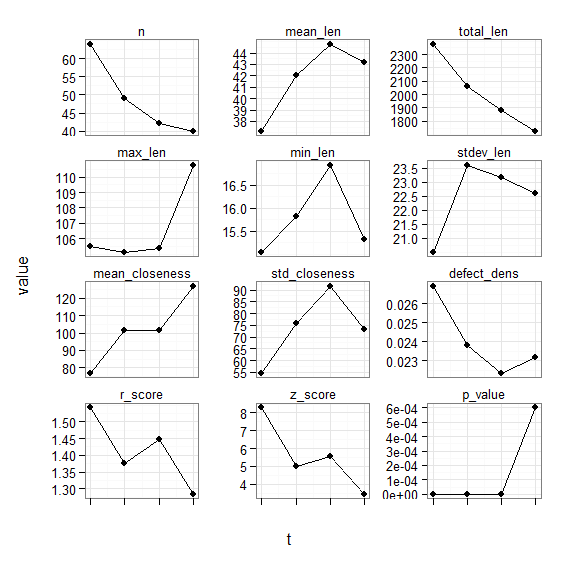
This code, combined with the data frame loading and melting above produced the following output:
Grid of plots (facet-based method)
That's a lot better, but still needs some tweaking. Members of the mailing list advised how to change the order of the plots, and I also found out how to remove variables that I didn't want. I then tweaked the appearance of the plot. The final task was to wrap the whole lot in a function called plot_graphs which takes an argument of the path to a CSV file and then plots the graphs based on it.
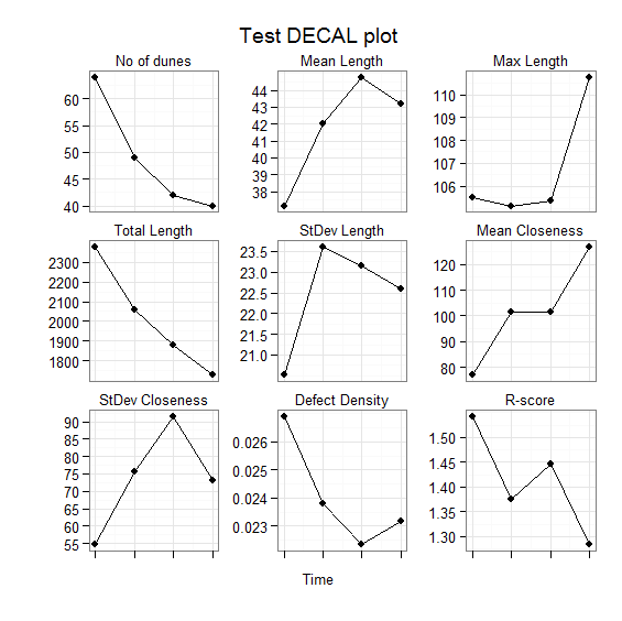
The final code is below, followed by the final output:
You'd think that would be the end of it...but the most useful part of this whole process was the advice given by members of the mailing list after I'd succeeded with my task.
This advice was a suggestion of a way of working within R and ggplot2 that will bring dividends: that is, to do as much of the data processing as possible outside ggplot2, and then just use simple graph plotting functions. R has loads of useful packages (like reshape which provides the melt command used above), and can do a lot of very clever processing very easily. Also, the ability of R to link to databases was mentioned, as SQL queries can often be a very good way to extract data for visualisation (something I may use to store dune metrics in a later version of DunesGIS).
So, thanks are due to all the members of the ggplot2 group who contributed to this 'journey of discovery': Baptiste, Dennis, Hadley, Brandon and Mark - thanks guys!
Well, I’ve finally solved a problem that I’ve been struggling with for days. On Friday my VPN connection to the University of Southampton was working fine, and then on Saturday it wouldn’t work. At that point, I assumed it was a problem at the university and waited until this morning to contact their IT support department. After a number of telephone calls we established that it was a problem with my computer, as other computers in my house could connect to the VPN fine. At this point they marked the issue as resolved and told me that I’d have to investigate it myself – which, although frustrating, I could understand.
While trying to solve this I did a lot of Google searches, and found a huge number of forum posts from people who were having VPN problems in Vista. Eventually, however, I found the result that helped me – and I’ve described the solution below.
Problem
Suddenly VPN connections in Vista stop working. When you try to connect to a VPN it sits for ages at the "Connecting to VPN" dialog, and then gives you Error 800 – VPN unreachable. However, even thought it says the VPN is unreachable, the VPN server can be pinged fine.
Solution
I eventually found a good solution on a forum (http://www.vistax64.com/vista-networking-sharing/112970-pptp-stopped-working.html). It involves running some commands on the command-line to uninstall and then reinstall the VPN drivers. So, firstly, open the command window (by clicking Start, typing cmd, and then pressing Enter) and type in the following lines, pressing enter after each one:
netcfg -u ms_l2tp
netcfg -u ms_pptp
netcfg -l %windir%\inf\netrast.inf -c p -i ms_pptp
netcfg -l %windir%\inf\netrast.inf -c p -i ms_l2tp
(that’s a lower-case letter L in the bottom two lines)
After running those commands, VPNs should be working again – hopefully! Let me know in the comments whether this works for you or not.
As part of my DunesGIS project I had a need to calculate ‘closeness statistics’ for objects in ArcGIS. By ‘closeness statistics’ I mean statistics giving information about how close the objects are to each other. I needed to do this to calculate how dune patterns change over time.
The code below takes a shapefile as input, and then calculates the closest other object to each object. It then returns the mean closeness and standard deviation of all objects.
def CalculateCloseness(Filename):
    # Calculate the distance from each shape (point, line, polygon)
    # to all of the others
    gp.GenerateNearTable(Filename, Filename, "NearTable", \
                         "", "LOCATION", "ANGLE", "ALL")

    # Create a view of the table so that we can run queries on it below
    gp.MakeTableView("NearTable", "tbl", "NEAR_DIST > 0")

    # Search for all of the distances which are > 175 and < 185 degrees
    # that is, basically horizontally
    rows = gp.SearchCursor("tbl", "NEAR_ANGLE >= 175 AND NEAR_ANGLE <= 185", "", "")

    # Get the first row
    row = rows.Next()

    # Create a NumPy array to hold the results
    shortest = numpy.zeros(500)

    # For each row
    while row:
        # Get the previous shortest distance from the array
        prev_value = shortest[row.IN_FID]

        # If the previous value is 0 then this is the first distance
        # we've found so set it to that
        if (prev_value == 0):
            shortest[row.IN_FID] = row.NEAR_DIST
            continue
        # Otherwise if this is a shorter one then use it
        elif (row.NEAR_DIST < prev_value):
            shortest[row.IN_FID] = row.NEAR_DIST

        # Move to the next row
        row = rows.Next()

    # Select all non-zero elements so the zero's don't skew the mean
    non_z_indices = numpy.where(shortest)

    # Calculate mean and stdev
    mean_closeness = numpy.mean(shortest[non_z_indices])
    std_closeness = numpy.std(shortest[non_z_indices])

    # Return results
    return [mean_closeness, std_closeness]
This script is (well, will shortly) be included in RTWTools for ArcGIS, where it is integrated into an ArcGIS Toolbox.
No, this isn’t about thinking deeply while the wind is blowing, or philosophising about how the wind is there but we can’t see it – it’s about sand dunes.
Now, you might think that sand dunes are quite boring things, just hills made out of sand that sit there and do nothing. That couldn’t be further from the truth. As I learnt in my Aeolian Geomorphology and Geomorphic Modelling course, sand dunes are complex, dynamic systems which do interesting things like move, merge, split, and even automatically organise themselves.
I’m doing some research on the self-organisation of sand dunes with Dr Jo Nield, and part of this research involves writing some software to automatically extract the crests of dunes from Digital Elevation Models (DEMs) showing an area of dunes (known as a dunefield), an example of which is shown in the image below), so that pattern metrics (statistics on the organisation of the dunes within the dune field) can be calculated. These DEMs are produced by a computer model which simulates dune field development. This software is being actively developed at the moment, and is available at my Dunes GIS page.
Example Digital Elevation Model (DEM) of a dune field
The issue that I want to write about today is the question what is a sand dune? It turns out that this question, which seems remarkably abstract, becomes very important when trying to write software to extract dune crests automatically – because to extract the crests of dunes you need to work out what is a dune and what isn’t! In fact, this problem often occurs when trying to write computer software to automate tasks that humans can do easily by hand. Academics who are manually tracing the crests of dunes from images on a computer screen have a large body of knowledge they can draw on to decide what is and isn’t a sand dune. Trying to program this knowledge into a computer is difficult, partly because it is often difficult to work out exactly what this body of knowledge contains.
If a human were to try to trace the crests of the dunes shown in the image above then he would struggle, as the image doesn’t show the crests of the dunes very clearly. In fact, the majority of the middle of the dune is shown as a single colour (bright red) – so it is difficult to tell where the actual crest is. Therefore, a sensible analyst would transform the image to look something like the image below.
A shaded relief version of the DEM
This transformation can be accomplished with one command in most image analysis software (if you’re interested I produced the above image in ENVI using the Topographic -> Topographic Modelling command) and shades the image so that it looks like a sun is shining on it from a certain direction. This makes the image look more ‘lifelike’, producing an image which is similar to the view you would get from an aircraft with the sun low in the sky) and therefore easier to interpret. The crests of the dunes can easily be seen, and therefore can be traced with a high accuracy.
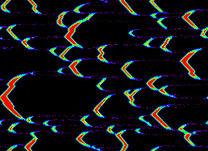
When implementing my automated method for tracing dunes I attempted to mirror the approach a human would use. Instead of using a shaded relief version of the DEM I used a similar version in which the values of each cell have a real-world meaning: the aspect map (shown below). Creating this image involves a simple process where each cell is assigned the direction that the slope of that cell faces (that is, its aspect) in degrees.
An aspect image created from the DEM above
As you can see, it is relatively easy to see where the dune crests are on this image. Therefore, it is relatively simple to write an algorithm to extract the dunes, by looking for the changes in colour on the image above (which are represented quantitatively by the shifting of the aspect value from less than 180 degrees to greater than 180 degrees).
However, this leads to a very messy set of crest lines, as much of the noise in the image is identified as a separate dune. When a human starts to trace dunes from this image their eye will be automatically drawn to some of the large dunes, and they will, almost subconsciously, ignore much of the noise which is visible in the image. A computer won’t do this, so therefore a number of filtering processes are used to both remove the noise before the image is processed, and remove the crests of ‘invalid’ dunes (for example, extremely short dunes) after the crests have been extracted.
But now the big question: are these crests that have been extracted actually the crests of real dunes? If we’re going to use this automated method to get statistics which can be used to develop scientific theories about the behaviour of sand dunes, then we’d better be pretty sure that the crests we’ve extracted actually belong to real dunes!
So, this all leads back to the question what is a sand dune? The answer, unsurprisingly, is not simple. I haven’t yet investigated all of the literature, but I remember learning in my aeolian geomorphology course that most models of dune formation require the dune to have three key characteristics before they can be said to be fully-developed sand dunes:
A gently sloping windward slope
A steeply sloping lee slope
Fully-developed grainflow and grainfall processes leading to dune movement
Note that the definition above mentions neither the existence of crests nor a minimum length for dunes. The existence of crests can be inferred from characteristics 1 and 2, as if these are present then there will be a crest. However, the presence of a crest does not necessarily mean that one slope is gentle and the other is steep. Also, the processes of dune movement are not, and in fact cannot, be identified from a single DEM. Therefore, it could be said that the existence of a crest is a necessary condition but not a sufficient condition for a dune to exist.
It can be seen from the above that the question what is a dune? is most definitely important when studying dunes, and also very difficult to answer. It also shows the limitations of using imperfect data to study the natural world. With access to the right data dunes could be identified with a very high confidence, but sadly this data is frequently unavailable. Therefore, information derived from imperfect data, using methods with unavoidable problems, is often used to develop scientific theories. This is obviously a problem, but is sadly often (or maybe always?) unavoidable.
I was chatting to someone the other day about the values in my life, and it led to a lot of thinking on my part. I decided to make two posts on my blog: one about my values in life generally, and one specifically about my academic values.
I think that the values below define what I am (or at least what I attempt to be) in the world of academia.
Openness
I will be open with information about my research. I will not attempt to hide information that I’ve found during my research: if it doesn’t work then I’ll say so. I will disseminate my research as widely as I can (both through peer-reviewed publications and through my website), to ensure that time is not wasted repeating research unnecessarily.
Repeatability
I will do my utmost to ensure that my research can be repeated as easily as possible as repeatability is one of the fundamental tenets of modern science. When I develop new algorithms I will release open-source implementations of them on GitHub. Where possible I will release the raw data that I used for each project on GitHub, my academic website or through the relevant journal’s online archive.
Clarity
I will do my utmost to be as clear as possible, allowing my research to be accessible to as many people as possible. Many times I have been frustrated by research which seems to have been made needlessly complicated, and I will endeavour not to do this. I will contribute to education about remote sensing by writing articles and blog posts about the subject in a clear and concise manner.
I’ve recently starting scripting ArcGIS using Python as part of one of my academic projects (about which I’ll post more later) and needed to be able to snap points to polylines – that is, move points so that they lie on the nearest polyline. An example would help to explain this:
In the image above, the black line is the relevant polyline, and the blue point is the original point. I wanted this point to lie on the line itself, which it did after processing (the red point).
A number of forum posts I read on the internet about this directed me to Hawth’s Tools for ArcGIS, but sadly these don’t work with ArcGIS 9.3, which is the version I am using. Instead, I wrote the Python code below which does the job using the ArcGIS Near (Analysis) command. The Python code is shown below, and is well commented so that it should be relatively easy to understand.
# ------ Snap Point to Line ------
# Author: Robin Wilson (robin@rtwilson.com)
# Description: Move the points in points so that they
#              lie on top of the nearest line
# --------------------------------
def snap_point_to_line(points, lines):
    # Load the Analysis toolbox so that the Near tool is available
    gp.toolbox = "analysis"

    # Perform the Near operation looking for the nearest line
    # (from the lines Feature Class) to each point (from the
    # points Feature Class). The third argument is the search
    # radius - blank means to search as far as is needed. The
    # fourth argument instructs the command to output the
    # X and Y co-ordinates of the nearest point found to the
    # NEAR_X and NEAR_Y fields of the points Feature Class
    gp.near(points, lines, "", "LOCATION"

    # Create an update cursor for the points Feature Class
    # making sure that the NEAR_X and NEAR_Y fields are included
    # in the return data
    rows = gp.UpdateCursor(points, "", "", "NEAR_X, NEAR_Y")

    row = rows.Next()

    # For each row
    while row:
        # Get the location of the nearest point on one of the lines
        # (added to the file as fields by the Near operation above
        new_x = row.GetValue("NEAR_X")
        new_y = row.GetValue("NEAR_Y")

        # Create a new point object with the new x and y values
        point = gp.CreateObject("Point")
        point.x = new_x
        point.y = new_y

        # Assign it to the shape field
        row.shape = point

        # Update the row data and move to the next row
        rows.UpdateRow(row)
        row = rows.Next()
This script is included in RTWTools for ArcGIS, where it is integrated into an ArcGIS Toolbox.
Last night I went to see a production of Alan Bennett’s The History Boys at the Oxford Playhouse. It was a very good production, and very thought-provoking in many respects (particularly useful for the Theory of Knowledge course my Dad teaches). I wanted to pick up on a particular line which occurs when one of the pupils talks about describing art "in other words", and the teacher responds immediately saying that surely the definition of art is that it cannot be described "in other words". This definition is what I want to investigate here.
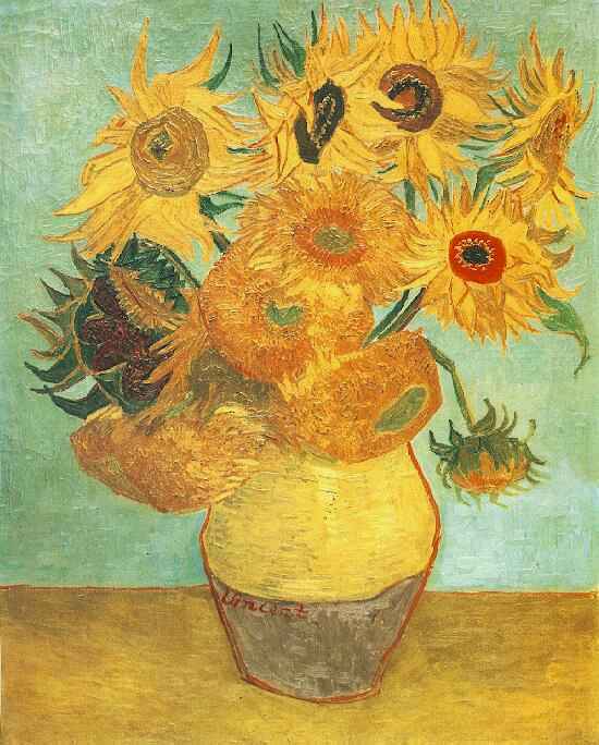
At first the definition seems very simple, rather obvious in fact (at least to me). Of course Van Gogh’s The Sunflowers can’t be described "in other words", in fact, it cannot really be described in words at all. It definitely can’t be described in other blobs of paint (at risk of sounding insulting to artists…) as then it wouldn’t be the piece of art that it is. But how about other types of art?
Van Gogh's Sunflowers
Can Beethoven’s Fifth Symphony be described "in other words", or even "in other sounds"? Well no, I would say that a description of the symphony in terms of the notes, the chords and the key changes is not a work of art: instead, it is a reduction of the art of composition to a simple listing ("stamp collecting", in the words of Rutherford). I was introduced to this concept at a young age (I think I must have been around eight at the time) when I composed my first piece of music (a very simple piece for piano). I wrote it down very carefully on manuscript paper and took it to show my Dad. "I don’t want to see it!" he said, "I want to hear it – it’s music, it needs to be heard to be appreciated" (even though my Dad can read music and hear it in his head easily).
Moving away from the visual arts…how about a poem? Can that be described "in other words"? One of the few poems I know relatively well (through studying it at GCSE) is Wilfred Owen’s Dulce et decorum est, an excerpt of which is below:
Bent double, like old beggars under sacks,
Knock-kneed, coughing like hags, we cursed through sludge,
Till on the haunting flares we turned our backs
And towards our distant rest began to trudge.
[…]
My friend, you would not tell with such high zest
To children ardentfor some desperate glory,
The old Lie; Dulce et Decorum est
Pro patria mori
That can’t be described in other words can it? The little excerpt doesn’t do it justice – read the whole thing, and think of the emotions it’s showing, and the powerful view on war expressed in the last stanza. Could I express that "in other words"?
Well, maybe I could. I could write something like the following:
It’s not nice being in the trenches. Seeing your friends die is horrible. In general, war is really horrible, so please don’t tell people it’s a good, honourable thing to do.
But that’s not art – that’s just a description of art, and it doesn’t do it justice at all. Reading what I just wrote makes you think "oh yeah, war’s not very nice really", reading Owen’s poem gives you a very different feeling.
The same could be said for other literary works. West Side Story is a very good retelling of Shakespeare’s Romeo and Juliet, but I’m sure Bernstein wouldn’t suggest that he’s trying to recreate Shakespeare "in other words". Yes, it is derived from Shakespeare, but it is not Shakespeare "in other words"
So, I’ve argued above that work produced in various fields generally taken to be "art" (various types of visual art and literature) cannot be described "in other words". But how about some other fields?
Take computer programming for example (see, everything in my life comes back to computers somewhere!). Can you describe a computing algorithm "in other words"? Yes, of course you can represent it differently, in different programming languages or using iteration instead of recursion (or vice versa), but surely it is still the same algorithm? Take the Quicksort algorithm – I can’t describe that in other words. Can you?
How about Fermat’s Last Theorem? Can you describe the question Fermat posed in any other words? No, at least not within our current mathematical system. In maths, and to a lesser extent in science, there is one way to describe something. Pythagoras’ Theorem has multiple proofs, but only one statement of what it is. Indeed, mathematical proofs should always be as simple as possible, based on other simple proofs, which in turn are based on more proofs which eventually lead back to axioms.
So, what does this mean? Is this a simple test as to whether something is an art? Well, maybe…
Computer programming is not generally considered an art, yet one of the pioneers of the field, Donald Knuth, wrote (and is indeed still writing) a series of books called The Art of Computer Programming. He obviously thinks it is, at least partially, an art.
How about maths? Although it is based entirely on simple logical steps, there is definitely an art to doing maths, and certain pieces of maths are definitely "works of art". Andrew Wiles’ proof of Fermat’s Last Theorem (described so well in Simon Singh’s book) is, in my opinion, just as much a "work of art" as a painting by Monet, or a novel by Jane Austen.
This is why I feel there is a problem with the black and white distinction between "arts" and "sciences". You find this a lot in education, at A-Level or University particularly. For example, most universities offer a BSc Geography degree (science-based) and a BA Geography degree (arts-based). However, is there not a significant amount of art in my BSc Geography degree? My (very efficient) code to calculate the Getis-Ord statistic on satellite images is, I believe, an artistic achievement.
I want to end this essay by asking you – what do you think? Do you think that the "in other words" test is a good test for whether something is an art? Is there a distinction between arts and sciences? How fuzzy is it? Can the "in other words" test be combined with a test for whether something is a science or not (Popper’s falsificationism comes to mind) to enable distinction between arts and sciences. If so, what happens when something can’t be described in other words, but is also falsifiable? Is it an art or a science? Or a ScArt (no, not the cable you use to connect your DVD player to your TV) or an Arence?
Comments are most definitely enabled on this post, and I would be very interested to hear what you’ve got to say.
It’s amazing what gets covered in lectures when you’re studying geography…
Today in my GEOG2006: Quaternary Environmental Change we were learning about extinctions during the Holocene (last 10,000 years ish). In a slight aside from the topic, while talking about the Black Rat (rattus rattus) and the Brown Rat (rattus something elseus) our lecturer (Tony Brown) told us that actually most of the evidence now points to rats not being involved in the bubonic plague in Britain.
Maps showing the extents of rat populations in the UK. Black rats on the left (mainly confined to coastal areas) and brown rats on the right
He suggests that various bits of evidence point towards this:
Rats move very slowly – at least compared to various other creatures. The bubonic plague spread from south east Kent to Derbyshire in about six months – the rats would have had to have been running for the entire six month period to get there that quickly!
The bubonic plague flea lives only on Black Rats. These are nowhere near as widespread as brown rats (in fact at the moment they’re on the endangered species list) and, as far as we know, have never been widespread in Britian – they only existed in small pockets around points of entry (normally ports like Southampton, Liverpool, London and Bristol).
It is almost possible to predict who in each village will get the bubonic plague – it seems to be almost always related to contact with other people. For example, the vicar and the doctor are likely to get it – even though they are likely to be relatively upper class and therefore less likely to have rats living in their houses.
Overall this seems to suggest that bubonic plague was an entirely human-spread contagious disease.
(NB: This entire post may be wrong. If so – it’s not my fault! I’m just reiterating information I heard from my lecturers…)