In 2019 I wrote about some of my favourite books I read that year and I never got round to doing a follow-up post with books from 2020, 2021 etc. Finally, in 2024 I’m actually going to write up some of these books.
I’ve read around 90 books since the start of 2020, and a lot of these were very good – so I’m going to do this post in a number of parts, so as not to overload you with too many great books at once.
So, part 1 is going to be the first chunk of non-fiction books that I want to recommend. I’ve tried to roughly categorise them, so, let’s get started with the first category:
Space books
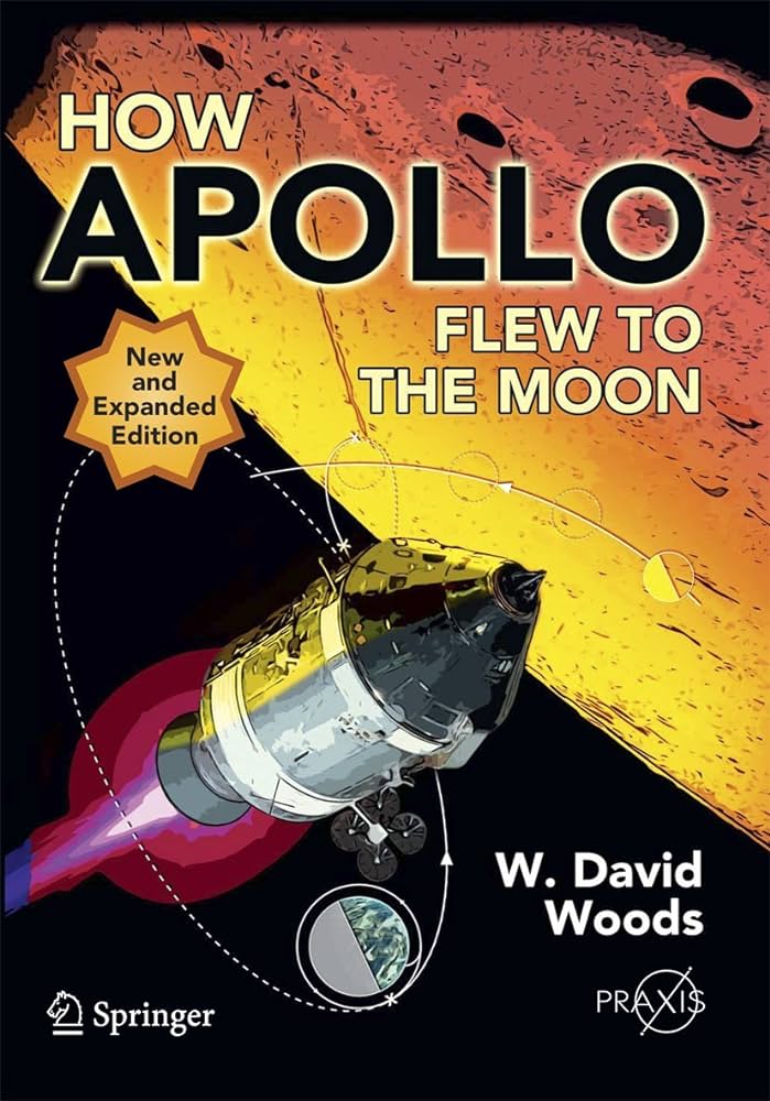
How Apollo Flew To The Moon by W. David Woods
Amazon link
This is an utterly fascinating book. It’s long, and it’s detailed – but that just makes it better (in my opinion). It covers a lot of technical detail about exactly how the Apollo missions and spacecraft worked – to literally answer the question of how they flew to the moon. All phases of flight are covered, from launch to splashdown, with details about each stage of countdown, how details of engine burns were passed to the crew (with worked examples!), how on-orbit rendezvous worked and more. It is liberally sprinkled with images and diagrams, and includes lots of quotes from the Apollo astronauts (from during the missions themselves, as well as from debriefs and trainings). This book is first on the list because it was genuinely one of the best books I’ve read – it was so fascinating and so well-written that I kept smiling broadly while reading it!
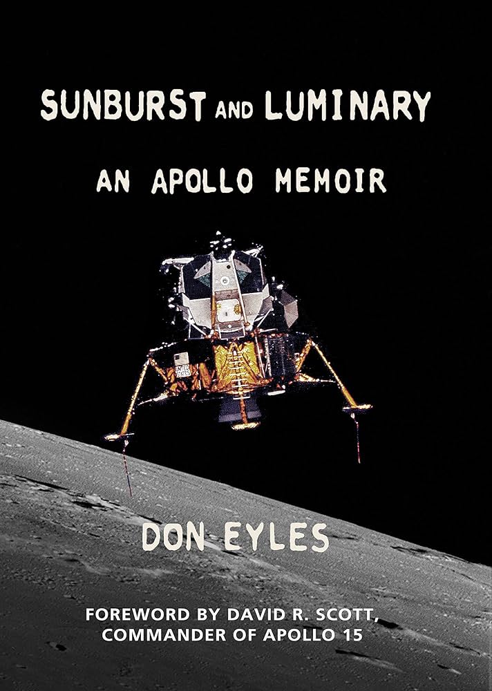
Sunburst and Luminary: An Apollo Memoir by Don Eyles
Amazon link
Another Apollo book now – but this time more concerned with the technicalities of the computing technology used during Apollo. The author was a computer programmer working on code for the lunar module computer, specifically the code used for the lunar landing itself. This book is definitely a memoir rather than pure non-fiction – it covers parts of the author’s life outside of Apollo – but that makes it less dry than some other books on Apollo computing (eg. Digital Apollo, which I never quite got into) but it still covers a lot of technical information. I never fail to be amazed by the complexity of the computing requirements for the Apollo missions, and how they managed to succeed with such limited hardware.
Into the Black by Rowland White
Amazon link
Now we turn our attention to the Space Shuttle. This book covers the first flight of the space shuttle and includes a massive amount of detail that I hadn’t known before. I won’t spoil too many of the surprises – but there was a lot more military involvement than I’d realised, and some significant concerns about the heat shield tiles (and this was decades before the Columbia accident). It’s very well written, with a lot of original research and quotes from the astronauts and original documents. Highly recommended.
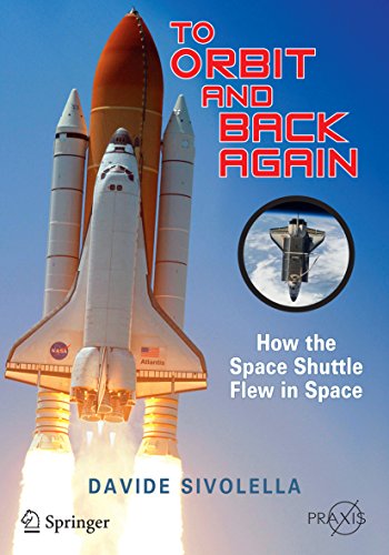
To orbit and back again: how the Space Shuttle flew in space by Davide Sivolella
Amazon link
This is the space shuttle equivalent of How Apollo Flew to the Moon. It is also fascinating, but not quite as well written, and therefore a bit harder to read. I got a bit lost in some of it – particularly the rendezvous parts – but the details on the launch, the computer systems, the environmental systems and tiles were fascinating.
Law books
This might be an unexpected category to find here, but I really enjoy reading books about law – mostly ones designed for lay-people. I’ve read all the typical books by people like the Secret Barrister – these are a few more unusual books.
What about law by Barnard, O’Sullivan and Virgo
Amazon link
This book has the subtitle ‘Studying Law at University’, but you can completely ignore that bit – it is a great book for anyone. With that subtitle you might expect it to cover how to choose a law course or the career progression for a lawyer – but instead, it ‘just’ gives a great introduction to all the major areas of UK law. It is absolutely fascinating. Chapters introduce law in general and the approach lawyers and law students take to the law, and then there are chapters for each major branch of UK law (criminal, tort, public, human rights etc). Each chapter then discusses the various principles of that branch of law and usually goes into detail on a few example cases. I found these examples to be the best bit – thinking about exactly what the law says when compared to the facts of the case, and what bits of law had to be decided by the judge or jury. It gave me a real appreciation for how much the law has to be "made up" (probably a bad choice of words) by the people interpreting it, as an Act of Parliament can never cover everything in enough detail. Note: Try and get the latest edition (3rd Ed at the time of writing) as there are interesting new bits about Brexit, and they cover the Supreme Court rather than the Law Lords.
Court Number One: The Old Bailey Trials that Defined Modern Britain by Thomas Grant
Amazon Link
This book gives a fascinating overview of various key trials that were held in the UK’s most famous courtroom – Court Number One at the Old Bailey. As well as talking about the trials themselves, the author covers the details of the case, and a lot about what life in Britain was like at the time of the trials, to give good context. I was really quite disturbed by the number of fairly obvious miscarriages of justice that were described here – but it was fascinating to hear the details (I’d heard of some of the cases before, but some were completely new to me).
The Seven Ages of Death by Richard Shepherd
Amazon link
This is a fascinating book, but you should be warned that it is quite upsetting at times, particularly in the chapter dealing with the deaths of babies and young children. I actually preferred this to Richard’s previous book (though I enjoyed both) – in this book he talks less about his personal history. Instead, he splits the book up into sections relating to different ages of people at their death. He talks very interestingly about the causes of death he sees at various different ages, and the general changes in people’s bodies that you’ll see at various ages (eg. bones that haven’t yet fused in children, damage due to drinking or smoking in middle age, changes in the bodies of elderly people). As well as discussing the bodies in detail, he also covers details of some of the cases, some of which are quite shocking.
Right, I think that’ll do for Part 1. Next time we’ll look at transport and Cold War books.
I came up with an interesting plan for an artistic map recently (more on that when I’ve finished working on it), and to create it I needed to be able to calculate a large number of driving routes around Southampton, my home city.
Specifically, I needed to be able to get lines showing the driving route from A to B for around 5,000 combinations of A and B. I didn’t want to overload a free hosted routing server, or have to deal with rate limiting – so I decided to look into running some sort of routing service myself, and it was actually significantly easier than I thought it would be.
It so happened that I’d come across a talk recently on a free routing engine called Valhalla. I hadn’t actually watched the talk yet (it is on my ever-expanding list of talks to watch), but it had put the name into my head – so I started investigating Valhalla. It seemed to do what I wanted, so I started working out how to run it locally. Using Docker, it was nice and easy – and to make it even easier for you, here’s a set of instructions.
Download an OpenStreetMap extract for your area of interest. All of your routes will need to be within the area of this extract. I was focusing on Southampton, UK, so I downloaded the Hampshire extract from the England page on GeoFabrik. If you start from the home page you should be able to navigate to any region in the world.
Put the downloaded file (in this case, hampshire-latest.osm.pbf) in a folder called custom_files. You can download multiple files and put them all in this folder and they will all be processed.
Run the following Docker command:
docker run -p 8002:8002 -v $PWD/custom_files:/custom_files ghcr.io/gis-ops/docker-valhalla/valhalla:latest
This will run the valhalla Docker image, exposing port 8002 and mapping the custom_files subdirectory to /custom_files inside the container. Full docs for the Docker image are available here.
You’ll see various bits of output as Valhalla processes the OSM extract, and eventually the output will stop appearing and the API server will start.
Visit http://localhost:8002 and you should see an error – this is totally expected, it is just telling you that you haven’t used one of the valid API endpoints. This shows that the server is running properly.
Start using the API. See the documentation for instructions on what to pass the API.
Once you’ve got the server running, it’s quite easy to call the API from Python and get the resulting route geometries as Shapely LineString objects. These can easily be put into a GeoPandas GeoDataFrame. For example:
import urllib
import requests
from pypolyline.cutil import decode_polyline

# Set up the API request parameters - in this case, from one point
# to another, via car
data = {"locations":[ {"lat":from_lat,"lon":from_lon},{"lat":to_lat,"lon":to_lon}],
        "costing":"auto"}
# Convert to JSON and make the URL
path = f"http://localhost:8002/route?json={urllib.parse.quote(json.dumps(data))}"
# Get the URL
resp = requests.get(path)
# Extract the geometry of the route (ie. the line from start to end point)
# This is in the polyline format that needs decoding
polyline = bytes(resp.json()['trip']['legs'][0]['shape'], 'utf8')

# Decode the polyline
decoded_coords = decode_polyline(polyline, 6)

# Convert to a shapely LineString
geom = shapely.LineString(decoded_coords)
Note that you need to pass a second parameter of 6 into decode_polyline or you’ll get nonsense out (this parameter tells it that it is in polyline6 format, which seems to not be documented particularly well in the Valhalla documentation). Also, I’m sure there is a better way of passing JSON in a URL parameter using requests, but I couldn’t find it – whatever I did I got a JSON parsing error back from the API. The urllib.parse.quote(json.dumps(data)) code was the simplest thing I found that worked.
This code could easily be extended to work with multi-leg routes, to extract other data like the length or duration of the route, and more. The Docker image can also do more, like load public transport information, download OSM files itself and even more – see the docs for more on this.
Check back soon to see how I used this for some cool map-based art.
This is a bit different to what I usually post on this blog (which is usually technical content about GIS, remote sensing, Python and data analysis – see afewexampleposts), and this is part of April Cools – a group of bloggers writing posts that are unusual for them, but still good content.
So, on that note, here are a few fairly simple recipes that we often make in our household. None of them are particularly fancy, but they all taste nice – and my family like them.
Sausage, apple and pepper thing – in the process of being cooked
Cheat’s Carbonara
Serves approx 3 people.
Chop chestnut mushrooms (half a tub) and bacon (approx. 4-6 rashers).
Fry bacon in a little oil, add mushrooms after a couple of minutes
Meanwhile, cook tagliatelle pasta in a separate saucepan, according to packet instructions
After about 5 minutes, add double-cream and a good sprinkling of pepper to the frying pan, and cook until the cream thickens and absorbs some of the bacon fat.
Mix in the cooked pasta, and serve with cherry tomatoes.
Cheat’s Curry
Serves approx 4 people.
Dice some chicken breast (or any other meat!), and fry until lightly browned
Add a tablespoon of curry paste (Korma paste or Thai Green Curry paste work well, but I imagine others would work too). Stir to coat.
Add a tin of coconut milk, stir to mix in the coconut solids. Add seasonings (mixed herbs, pepper, salt) to taste.
Cook until sauce thickens, and serve with rice
Optional: Add diced peppers or other vegetables to the pan at the start.
Coronation Rice
(lovely as a side for a picnic or barbeque)
Put a heaped spoonful of turmeric into a saucepan full of water, and cook rice in the saucepan according to the packet instructions.
Drain rice and cool under running cold water
Cut up dried apricots into very small pieces, and mix these and a few handfuls of sultanas into the rice
Add curry power, mayonnaise and mango chutney to the bowl and stir until well-mixed (you may find it easier to mix these three ingredients separately and then add to the main bowl once combined)
Refrigerate and leave to develop a deeper flavour.
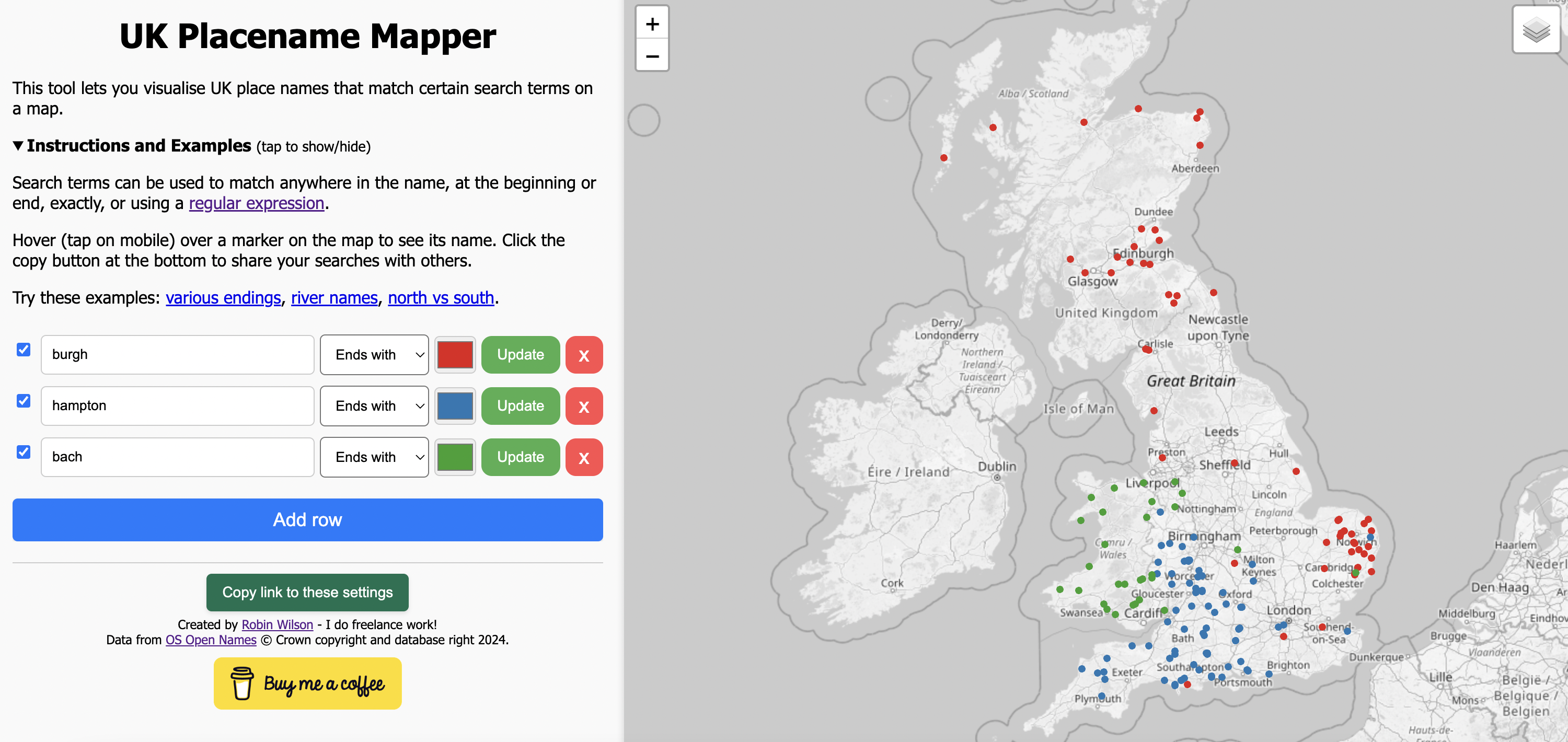
As an Easter present for you all, I’ve got a new web app you can play with.
It lets you search for UK place names – things like ‘ends with burgh’ or ‘starts with great’ or ‘contains sea’ – and then plot them on an interactive map. Once you’ve done that, you can even share links to your settings so other people can see your findings.
Have a look at the web app now, and please tweet/toot/email me with any interesting things you find.
The data comes from the Ordnance Survey Open Names dataset, and it was processed on my local machine using Python to create some filtered data that could be used in the webapp, which all runs client-side.
This is only about 3 years late – but I gave a talk at FOSS4G 2021 on geospatial PDFs. The full title was:
From static PDFs to interactive, geospatial PDFs, or, ‘I never knew PDFs could do that!’
The video is below:
In the talk I cover what a geospatial PDF is, how to export as a geospatial PDF from QGIS, how to import that PDF again to extract the geospatial data from it, how to create geospatial PDFs using GDAL (including styling vector data) – and then take things to the nth degree by showing a fully interactive geospatial PDF, providing a UI within the PDF file. Some people attending the talk described it as "the best talk of the conference"!
Here’s a bit of SQL I wrote recently that had an error in it which I struggled to find. The error I got was ERROR: invalid reference to FROM-clause entry for table "roads" and I did some Googling but nothing really seemed to make sense as a cause of this error.
My SQL looked like this:
WITH args AS (
    SELECT
        ST_TileEnvelope(z, x, y) AS bounds,
        ST_Transform(ST_MakeEnvelope(l, b, r, t, 4326), 27700) AS area
),
mvtgeom AS (
    SELECT
        ST_AsMVTGeom(
            ST_Transform(ST_Intersection(roads.geom, args.area), 3857),
            args.bounds
        ) AS geom
    FROM
        roads, args
    JOIN floods ON ST_Intersects(roads.geom, floods.wkb_geometry)
    WHERE
        roads.geom && args.area
        AND roads.geom && args.bounds
)
SELECT
    ST_AsMVT(mvtgeom, 'default') INTO result
FROM
    mvtgeom;
This looks a bit weird, but it’s a slightly re-written version of the SQL inside a function that was written to produce Mapbox Vector Tiles (MVT) for use in an online webmap. The function is picked up by pg_tileserv and called appropriately when tiles are needed.
What I’m doing in the code is setting up a couple of parameters – the tile envelope and the selected area, and then running a fairly simple join with extra WHERE conditions, converting the outputs to MVT geometries and then the whole thing to a MVT itself.
The problem is inside the mvtgeom AS section – let’s simplify the SQL there a bit so it is easier to look at:
SELECT
        ST_Intersection(roads.geom, args.area), 3857) AS geom
FROM
        roads, args
        JOIN floods ON ST_Intersects(roads.geom, floods.wkb_geometry)
WHERE
        roads.geom && args.area
        AND roads.geom && args.bounds
I’ve got rid of all the MVT related stuff, so we have a more standard PostGIS query: we’re looking for the intersection of the roads and the area, where the roads intersect the floods, and the roads are inside the area and inside the tile boundaries (both defined in the args CTE). Possibly the error is a bit clearer now – maybe…
The answer is, it’s all about the placement of the JOIN clause. I’d never really properly thought about this (even though it’s a bit obvious!), but the JOIN statement refers to the table listed immediately before it. Therefore, if we reformat the above slightly we’re selecting:
FROM
roads,
args JOIN floods ON ST_Intersects(roads.geom, floods.wkb_geometry)
That is, we are running the JOIN on the args table, not on the roads table. The slightly confusing error message (ERROR: invalid reference to FROM-clause entry for table "roads" ) means that this JOIN clause makes no sense when run against the args table, as there’s no such thing as roads in that context.
All we need to do to fix this is move the JOIN clause before args:
FROM
roads JOIN floods ON ST_Intersects(roads.geom, floods.wkb_geometry),
args
Remember the comma after the JOIN clause – we’re still in the list of tables/things that we’re selecting FROM.
In general, the format of a FROM clause is:
FROM
<tablename> [JOIN clause],
<tablename>,
…
For context, I was running this SQL in Postgres, with the PostGIS extension. I’m not an expert in SQL, so please let me know if I’ve made any errors in this post.
Summary: It might be because there is an exception raised when importing your function_app.py – for example, caused by one of your import statements raising an exception, or a parsing error caused by a syntax error.
I was deploying a FastAPI app to Azure Functions recently. Azure Functions is the equivalent of AWS Lambda – it provides a way to run serverless functions.
Since I’d last used Azure Functions, Microsoft have introduced the Azure Functions Python V2 programming model which makes it easier and cleaner to do a number of common tasks, such as hooking up a FastAPI app to run on Functions.
However, it also led to an error that I hadn’t seen before, and that I couldn’t find documented very well online.
Specifically, I was getting an error at the end of my function deployment saying No HTTP triggers found. I was confused by this because I had followed the documented pattern for setting up a FastAPI app. For reference, my function_app.py file looked a bit like this:
import azure.functions as func
from complex_fastapi_app import app

app = func.AsgiFunctionApp(app=app,
            http_auth_level=func.AuthLevel.ANONYMOUS)
This was exactly as documented. But I kept getting this error – why?
I replaced the import of my complex_fastapi_app with a basic FastAPI app defined in function_app.py, this time copied directly from the documentation:
Everything worked fine now and I didn’t get the error.
After a lot of debugging, it turns out that if there is an exception raised when importing your function_app.py file then Functions won’t be able to establish what HTTP triggers you have, and will give this error.
In this case, I was getting an exception raised when I imported my complex_fastapi_app, and that stopped the whole file being processed. Unfortunately I couldn’t find anywhere that this error was actually being reported to me – I must admit that I find Azure logging/error reporting systems very opaque. I assume it would have been reported somewhere – if anyone reading this can point me to the right place then that’d be great!
I’m sure there are many other reasons that this error can occur, but this was one that I hadn’t found documented online – so hopefully this can be useful to someone.
Summary: If appending to a PostGIS table with GDAL/OGR is taking a long time, try setting the PG_USE_COPY config option to YES (eg. adding --config PG_USE_COPY YES to your command line). This should speed it up, but beware that if there are concurrent writes to your table at the same time as OGR is accessing it then there could be issues with unique identifiers.
As with many of my blog posts, I’m writing this in the hope that it will appear in searches when someone else has the same problem that I ran into recently. In the past I’ve found myself Googling problems that I’ve had before and finding a link to my blog with an explanation in a post that I didn’t even remember writing.
Anyway, the problem I’m talking about today is one I ran into when working with a client a few weeks ago.
I was using the ogr2ogr command-line tool (part of the GDAL software suite) to import data from a local Geopackage file into a PostGIS database (ie. a PostgreSQL database with the PostGIS extension).
I had multiple files of data that I wanted to put into one Postgres table. Specifically, I was using the lovely data collated by Alasdair Rae on the resources page of his website. Even more specifically, I was using some of the Local Authority GIS data to get buildings data for various areas of the UK. I downloaded multiple GeoPackage files (for example, for Southampton City Council, Hampshire County Council and Portsmouth City Council) and wanted to import them all to a buildings table.
I originally tested this with a Postgres server running on my local machine, and ran the following ogr2ogr commands:
Here I’m using the -f switch and the arguments following it to tell ogr2ogr to export to PostgreSQL and how to connect to the server, giving it the input file of buildings1.gpkg and using the -nln parameter to tell it what layer name (ie. table name) to use as the output. In the second command I do exactly the same with buildings2.gpkg but also add -append and -update to tell it to append to the existing table rather than overwriting it.
This all worked fine. Great!
A few days later I tried the same thing with a Postgres server running on Azure (using Azure Database for PostgreSQL). The first command ran fine, but the second command seemed to hang.
I was expecting that it would be a bit slower when connecting to a remote database, but I left it running for 10 minutes and it still hadn’t finished. I then tried importing the second file to a new table and it completed quickly – therefore suggesting it was some sort of problem with appending the data.
I worked round this for the time being (using the ogrmerge.py script to merge my buildings1.gpkg and buildings2.gpkg into one file and then importing that file), but resolved to get to the bottom of it when I had time.
Recently, I had that time, and posted on the GDAL mailing list about this. The maintainer of GDAL got back to me to tell me about something I’d missed in the documentation. This was that when importing to a brand new table, the Postgres COPY mode is used, but when appending to an existing table individual INSERT statements are used instead, which can be a lot slower.
Let’s look into this in a bit more detail. The PostgreSQL COPY command is a fast way of importing data into Postgres which involves copying a whole file of data into Postgres in one go, rather than dealing with each row of data individually. This can be significantly faster than iterating through each row of the data and running a separate INSERT statement for each row.
So, ogr2ogr hadn’t hung, it was just running extremely slowly, as inserting my buildings layer involved running an INSERT statement separately for each row, and there were hundreds of thousands of rows. Because the server was hosted remotely on Azure, this involved sending the INSERT command from my computer to the server, waiting for the server to process it, and then the server sending back a result to my computer – a full round-trip for each row of the table.
So, I was told, the simple way to speed this up was to use a configuration setting to turn COPY mode on when appending to tables. This can be done by adding --config PG_USE_COPY YES to the ogr2ogr command. This did the job, and the append commands now completed nice and quickly. If you’re using GDAL/OGR from within a programming language, then have a look at the docs for the GDAL bindings for your language – there should be a way to set GDAL configuration options in your code.
The only final part of this was to understand why the COPY method isn’t used all the time, as it’s so much quicker. Even explained that this is because of potential issues with other connections to the database updating the table at the same time as GDAL is accessing it. It is a fairly safe assumption that if you’re creating a brand new table then no-one else will be accessing it yet, but you can’t assume the same for an existing table. The COPY mode can’t deal with making sure unique identifiers are unique when other connections may be accessing the data. whereas individual INSERT statements can cope with this. Therefore it’s safer to default to INSERT statements when there is any risk of data corruption.
As a nice follow-up for this, and on the maintainer’s advice, I submitted a PR to the GDAL docs, which adds a new section explaining this and giving guidance on setting the config option. I’ve copied that section below:
When data is appended to an existing table (for example, using the -append option in ogr2ogr) the driver will, by default, emit an INSERT statement for each row of data to be added. This may be significantly slower than the COPY-based approach taken when creating a new table, but ensures consistency of unique identifiers if multiple connections are accessing the table simultaneously.
If only one connection is accessing the table when data is appended, the COPY-based approach can be chosen by setting the config option PG_USE_COPY to YES, which may significantly speed up the operation.
I ran into a situation recently where I needed to create a Windows 10 bootable USB stick. I could easily download a Windows 10 ISO file, but I knew that it needed some ‘special magic’ to write it to a USB stick that would boot properly.
I tried various solutions (including windiskwriter) but none of them worked – until I tried Ventoy.
I got rather confused when reading the Ventoy webpage, so I wanted to write a quick blog post to show how to use it for this specific use case. The technology I had available to me was one M1 MacBook Pro running macOS and one x64 desktop machine with no OS (on which I wanted to install Windows) – and so these instructions will be based around this situation.
The way that Ventoy works is that you write the Ventoy image to a USB stick and it creates multiple partitions: some boot partitions, plus a big empty partition using up most of the space on the USB stick. You then copy your boot ISO files (for Windows, or Linux or whatever) onto that partition. When you boot from the USB stick Ventoy will provide a menu to allow you to pick an ISO, and then it will boot that ISO as if it had been burned to the USB stick itself. The easiest (and most reliable) way to write the Ventoy image to a USB stick is to use a bootable Ventoy image to do it – a double-USB-stick approach.
Burn that to a USB stick (it can be a small one) using a standard USB stick burning program like balenaEtcher
Boot from that USB stick on my x64 machine.
Insert another USB stick (ideally a fairly large one) into that machine (while keeping the first one inserted) and follow the on-screen instructions to burn Ventoy to that USB stick.
Shutdown that computer
Insert that USB stick into my Mac, and copy the Windows 10 ISO file onto the large empty partition.
Boot from that USB stick on the x64 computer. It will show an interface to allow you to choose an ISO to boot – there will be only one, so just press Enter. A few minutes later the Windows 10 installer will be ready to use.
Of course you can now keep this Ventoy USB stick around, and add other ISO files to it as needed.
I use GeoPandas for a lot of my vector GIS data manipulation in Python.
I had a situation the other day where I ended up with duplicates of some geometries in my GeoDataFrame, and I wanted to remove them. The simple way to do this is to use the underlying pandas method drop_duplicates on the geometry column, like:
gdf.drop_duplicates('geometry')
However, even after running this I still had some duplicate geometries present. I couldn’t quite believe this, so checked multiple times and then started examining the geometries themselves.
What I found was that my duplicates were technically different geometries, but they looked the same when viewing them on a map. That’s because my geometries were LineStrings and I had two copies of the geometry: one with co-ordinates listed in the order left-to-right, and one in the order right-to-left.
This is illustrated in the image below: both lines look the same, but one line has the individual vertex co-ordinates in order from left-to-right and one has the same co-ordinates in order from right-to-left.
These two geometries will show as the same when using the geometry.equals() method, but won’t be picked up by drop_duplicates. That’s because drop_duplicates just serialises the geometry to Well-Known Binary and compares those to check for equality.
I started implementing various complex (and computationally-intensive) ways to deal with this, and then posted an issue on the GeoPandas Github page. Someone there gave me a simple solution which I want to share with you.
All you need to do is run gdf.normalize() first. So, the full code would be:
gdf.normalize()
gdf.drop_duplicates('geometry')
The normalize() method puts the vertices into a standard order so that they can be compared easily. This works for vertex order in lines and polygons, and ring orders in complex polygons.